Kerala Plus Two Microeconomics Chapter Wise Questions and Answers Chapter 3 Production and Costs
Plus Two Economics Production and Costs One Mark Questions and Answers
Question 1.
Which among the following cost curves is not ‘U’ shaped?
Answer:
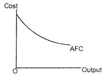
AFC curve is rectangular hyperbola.
Question 2.
Identify the shape of the following AFC curve?
Answer:
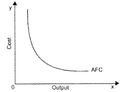
The shape of AFC curve is rectangular hyperbola.
Question 3.
When a firm increased the number of labour from 10 to 11, keeping the capital fixed the total product increased from 120 to 130. Which of the following statement is correct in this regard?
(a) The total product fell
(b) This is a long run production
(c) The average product is rising
(d) 10 is the marginal product of an increased unit of labour.
Answer:
(d) 10 is the marginal product of an increased unit of labour.
Question 4.
Slope of an isoquant is:
(a) marginal cost
(b) DMRS
(c) DMRTS
(d) None of the above
Answer:
(c) DMRTS
Question 5.
When MP becomes zero, TP:
(a) increases
(b) decreases
(c) becomes maximum
(d) becomes negative
Answer:
(c) becomes maximum
Question 6.
Which among the following is not ‘u’ shape
(a) MC
(b) AC
(c) AVC
(d) AFC
Answer:
(d) AFC
Question 7.
When AC is minimum
(a) MC > AC
(b) MC = AC
(c) MC < AC
(d) None of these
Answer:
(b) MC = AC
Question 8.
All the following curves are U shaped except
(a) the AVC curve
(b) the AFC curve
(c) the AC curve
(d) the MC curve
Answer:
(b) the AFC curve
Plus Two Economics Production and Costs Two Mark Questions and Answers
Question 1.
Let the production function of a firm be Q = 5 L1/2 K1/2
Find the maximum output that the firm can produce with 100 units of L and 100 units of K.
Answer:
The production function is
Q = 5 L1/2 K1/2
Since the firm uses 100 units of L and 100 units of
K, we get the production function as
Q = 5 × 1001/2 1001/2
Q = 5 × 10x 10
Q = 5 × 100 = 500
Question 2.
Derive marginal product and average product from the total product schedule.
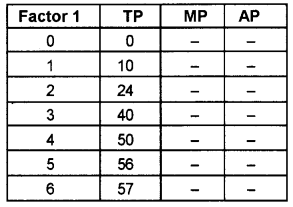
Answer:
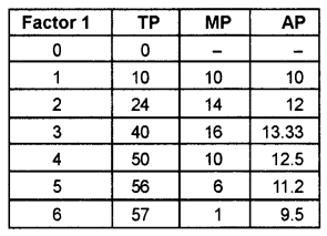
Question 3.
Find the maximum possible output for a firm with zero units of labour and 10 units of capital when its production function is
Q = 5L + 2K
Answer:
The production function is Giving the values of L and K, we get
Q = 5 × 0 + 2 × 10
Q = 0 + 20 = 20
Question 4.
“In the long run, all costs are variable”. Do you agree? Justify your answer.
Answer:
Yes. In the long run, all costs are variable. This is because there is sufficient time available in the long run for any factor of production to get increased. As there are only variable factors, in the long run, all costs are variable.
Question 5.
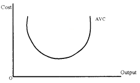
“The AVC is U shaped” explain the reasons for the ‘U’ shape of AVC curve. Also, draw a diagram to clarify your points.
Answer:
The SMC and AVC curves start rising when production starts. As output increases, SMC falls. AVC being the average of marginal costs also falls but falls less than SMC. Then after a point, SMC start rising. AVC, however, continues to fall as long as value of SMC remains less than the prevailing value of AVC.
Once the SMC has risen sufficiently its value becomes greater than the value of AVC. The AVC starts rising. Therefore, the AVC curve is “U” shaped. It is given in the following diagram.
Question 6.
TFC of a firm is ₹2,000 and TVC is ₹3,000. It produces 20 units. Calculate the AVC and AC of the firm.
Answer:
TC = TFC + TVC
AC = 5000/20 = 250
AVC = 3000/20 = 150
Question 7.
Can there be some fixed cost in the long run?
Answer:
No, there cannot be some fixed cost in the long run. This is because, in the long run all factors of production can be adjusted and variable.
Question 8.
Let the production function of a firm be Q = 10 L1/2 K1/2 Find out the maximum possible output that the firm can produce with 100 units of L and 100 units of K.
Answer:
The production function is,
Q = 10 L1/2 K1/2
L =100 units
K =100 units
∴ Q = 10 × 1001/2 × 1001/2
= 10 × (10²)1/2 × (10²)1/2
= 10 × 10 × 10
= 1,000 units
Question 9.
The table given below shows the total product schedule of labour. Determine the AP and MP of labour?
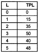
Answer:
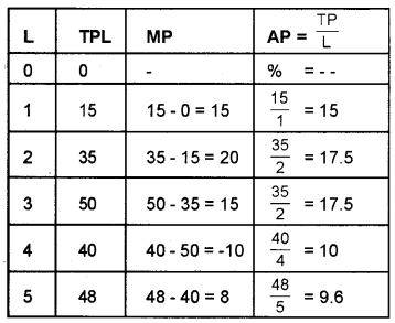
Question 10.
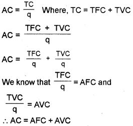
Prove that AC is the sum of AFC and AVC.
Answer:
Question 11.
A bus company started its operation with two buses, four labourers. It has paid a one-time road tax. As the passengers increased the company arranged more tripes, with the help of additional labour and for using more fuels. Classify the costs incurred by the bus company into fixed and variable.
Answer:

Question 12.
Both short run and long run average and marginal cost curves are U-shaped. But reasons for the U-shape are not the same. Bring out the differences.
Answer:
Behaviour of output in the short run as explained by the law of variable proportions Behaviour of output in the long run as explained by the laws of returns to scale.
Plus Two Economics Production and Costs Three Mark Questions and Answers
Question 1.
Match the following.
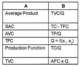
Answer:
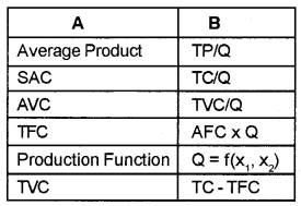
Question 2.
Categorize the following into fixed cost
(a) wages of temporary workers
(b) cost of raw materials
(c) salary of permanent staff
(d) cost of transportation
(e) cost of plant
Answer:
| Fixed Cost | Variable Cost |
| Salary of permanent staff | Cost of raw materials |
| Cost.of acquiring land | Cost of transportation |
| Cost of plant | Wages of temporary workers |
Question 3.
Identify the following curves.
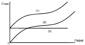
Answer:
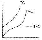
- TC
- TVC
- TFC
Question 4.
Identify the shapes of the following cost curves.
- AFC
- AC
- TFC
- TVC
- TC
Answer:
- AFC – Rectangular hyperbola
- AC – ‘U’shape
- TFC – Straight line parallel to X axis
- TVC – Inverse‘S’ shape
- TC – Inverse‘S’ shape
Question 5.
There exists vertical distance between 1. TVC and TC and (b) TC and TFC. What does this distance indicate?
- TVC and TC
- TC and TFC
Answer:
- The vertical distance between TVC and TC represents the Total Fixed Costs (TFC).
- The vertical distance between TC and TFC represents the Total Variable Costs (TVC)
Question 6.
Complete the following table
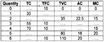
Answer:
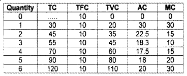
Question 7.
Name the following curves. ,
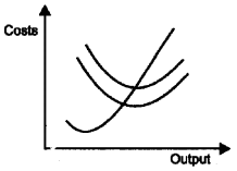
Answer:
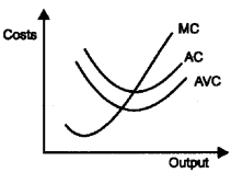
Question 8.
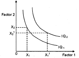
What do you mean by an ‘isoquant’?
Answer:
An isoquant is the set of all possible combinations of the two inputs that yield the same maximum possible level of output. Each isoquant represents a particular level of output and is labelled with that amount of output. The shape of isoquant is drawn below.
Question 9.
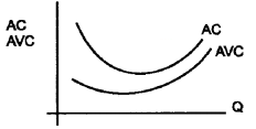
With the help of a diagram show the relation between average exists and average variable cost.
Answer:
Both AC and AVC are U shaped. As the output increases the gap between AC and AVC narrows.
Question 10.
In the short run, Total Variable Cost is zero when output is zero. When output rises, Total Cost also rises. Draw a suitable diagram and explain the relationship between Total Fixed Cost, Total Variable Cost and Total Cost.
Answer:
Question 11.
“Average Fixed Cost (AFC) curve is a continuously falling curve.”
- Substantiate this statement by giving the reasons.
- Graphically represent the AFC curve
Answer:
1. TFC is constant & hence AFC falls
2.
Plus Two Economics Production and Costs Five Mark Questions and Answers
Question 1.
The marginal product and total product of input are related’. Prove this statement.’
Answer:
The marginal product (MP) and total product (TP) of input are related. The points of the relationship are given below.
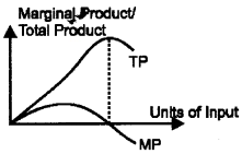
- When MP increases, TP also increases
- When MP is zero, TP becomes maximum
- When MP becomes negative, TP turns negative
Question 2.
Differentiate between returns to a factor and returns to scale.
Answer:
Returns to a factor refers to the effects on output of changes in one input with all other inputs are hold constant. On the other hand, returns to scale refers to the effect on total output of charges in some constant rate in all the inputs simultaneously.
Question 3.
The marginal cost and average cost are related to each other. Prove this using diagram and a numerical example?
Answer:
Marginal cost are addition made to the total costs by the production of an additional unit of the commodity.
MC = TCn – TCn-1
Average lost is per unit cost of production which is obtained by dividing the total cost by number of units of output produced.
\(A C=\frac{T C}{Q}\)
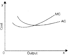
Since AC is obtained by dividing TC by all units, MC is the addition to TC by producing an additional unit so MC brings a change in AC.
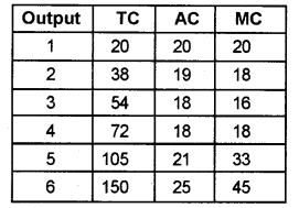
From above:
- When MC is less than AC, then MC will fall
- When MC is equal to AC, AC remains costant.
- When MC is more than AC, AC rises
Question 4.
Which of the following represent the long run production function?
1. MC is less than AC, then MC will fall
- Law of variable proportion
- Returns to scale
2. Explain what may happen when all inputs vary simultaneously?
Answer:
Returns to scale.
When all inputs are varied simultaneously the output may change in three ways.
1. Constant returns to scale:
It is when a proportional increase in inputs result in an increase in output by the same proportion.
2. Increasing returns to scale:
It is when a proportional increase in all inputs result in an increase in output by more than proportion.
3. Decreasing returns to scale:
It is when a proportional increase in all inputs result in an increase in output by less than proportion
Question 5.
State whether the statement are true or false.
- TC never becomes zero.
- AC is sum total of AFC and AVC.
- When AC rises, AC and MC are equal
- Real cost is the cost in money terms
- TFC curve is U shaped
Answer:
- True
- True
- False
- False
- False
Question 6.
The following table shows the total cost schedule of a firm. What is the total fixed cost schedule of the firm? Calculate the JVC, AFC, AVC, SAC and SMC of the firm
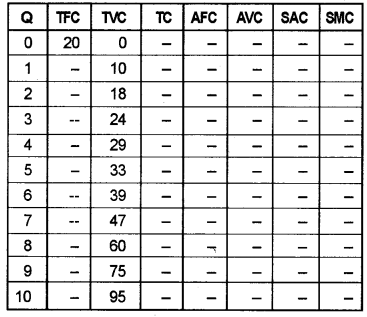
Answer:
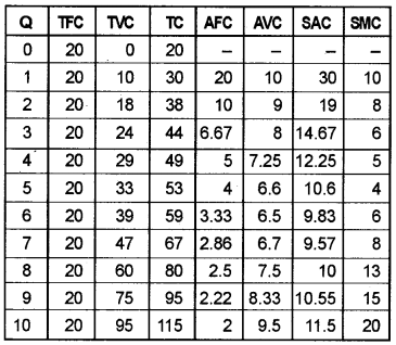
Question 7.
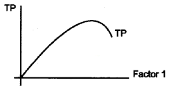
The diagram shows the total product curve of a factor in the law of variable proportion.
- Explain the law
- With the help of a diagram illustrate the average and marginal product curve and their relation.
Answer:
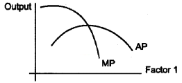
1. Law of variable proportion says that if one variable input is added with other fixed inputs the marginal product of a factor input initially rises but after reaching a certain level of output it starts falling.
2. The relation between the average and marginal product is given below. BothAPand MPare ‘n ’shaped. MPwill always pass through the maximum of AP.
Question 8.
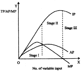
Theory of production deals with producer’s behaviour, and according to this theory output produced by a firm passes through three stages in the short run.
- Which are the three stages of production?
- Analyse and bring out the salient features of each stage.
- Which stage of production is very important as far as a firm is concerned? Why?
- Give suitable diagram by drawing the Total Prod-uct, Average Product & Marginal Product curves.
Answer:
1. Increasing, diminishing and negative
2. First output increases at increasing rate, then at diminishing rate & finally starts falling.
3. Second stage, profit maximisation occurs in this Stage.
4.
Question 9.
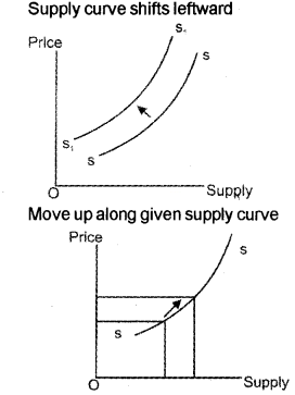
If other things remaining same, graphically explain what happens to the supply curve for readymade shirts if there is
- An increase in the wages paid to the tailors.
- An increase in the price of ready-made shirts
Answer:
Plus Two Economics Production and Costs Eight Mark Questions and Answers
Question 1.
Prepare a seminar report on the topic “Production Function.”
Answer:
Respected teachers and dear friends:
The topic of my seminar paper is “Production Function”. The production function of a firm shows relationship between inputs and output. In this seminar paper, I would like to present the different production functions such as short run production function and the long run production function.
Introduction:
As we know the production function shows the transformation of inputs into output. The production function can be of two types – short run production function known as Law of Variable proportion and the long run production function known as returns to scale. Q =F(F1 F2… Fn)
Contents:
A. Law of Variable proportion
- Increasing returns
- Diminishing returns
- Negative returns
A. The Law of Variable Proportions
When more and more units of a variable input are added with the fixed input, the marginal product would increase only upto a certain point. Therefore, the marginal product declines. This phenomenon is known as the Law of Variable Proportions. It is also known as returns to a factor.
The shape of TP, AP and MP suggests that they are specifically passing through three phases.
They are:
1. First phase:
In the first stage, both AP and MP increase. As a result TP also increases at an increasing rate. This stage is known as the stage of increasing return to a factor. AP reaches the maximum level in this stage.
2. Second phase:
Both AP and MP decrease at this stage. The TP increases at a decreasing rate. More importantly, TP reaches maximum and MP touches zero. This stage is also known as the stage of diminishing returns to a factor.
3. Third phase:
At this stage, the MP becomes negative. As a result, TP also starts declining. The decline of AP is continuous. In the graph, when TP reaches maximum and MP touches zero. When MP becomes negative, TP starts declining. This stage is known as the stage of negative returns to a factor.
B. Returns to scale
- Increasing returns
- Constant returns
- Decreasing returns
(for details, refer summary part)
B. Returns to scale
As stated earlier, all the factor inputs become variable in the long run and thereby no distinction can be made between fixed inputs and variable inputs. Return to scale is associated with long run production function.
Returns to scale refers to the change in output when all inputs are variable and the proportion between inputs remains constant. When all the inputs vary in the same proportion, the output (TP) behaves in different manner, which can be clubbed into three categories.
1. Increasing Returns to Scale (IRS):
When a proportionate change in all the inputs leads to more than proportionate change in output, it is known as the stage of increasing returns to scale. For instance, a 10% change in inputs results in more than 10% change in output.
2. Constant Returns to Scale (CRS):
When a proportionate change in all the inputs leads to change in output in the same proportion is known as the stage of constant returns to scale. It indicates that a 10% change in inputs leads to exactly 10% change in output.
3. Decreasing Returns to Scale (DRS):
When a proportionate change in all the inputs leads to less than proportionate change in output is known as the stage of decreasing returns to scale. It indicates that a 10% change in inputs leads to less than 10% change in output.
Conclusion:
Thus it can be concluded that there are two types of production function depending upon the use of inputs and the time period.
Question 2.
Prepare a seminar paper on Law of Returns to Scale.
Answer:
Returns to scale:
As stated earlier, all the factor inputs become variable in the long run and thereby no distinction can be made between fixed inputs and variable inputs. Return to scale is associated with long run production function.
Returns to scale refers to the change in output when all inputs are variable and the proportion between inputs remains constant. When all the inputs vary in the same proportion, the output (TP) behaves in different manner, which can be clubbed into three categories.
1. Increasing Returns to Scale (IRS):
When a proportionate change in all the inputs leads to more than proportionate change in output, it is known as the stage of increasing returns to scale. For instance, a 10 percentage change in inputs results in more than 10 percentage change in output.
2. Constant Returns to Scale (CRS):
When a proportionate change in all the inputs leads to change in output in the same proportion is known as the stage of constant returns to scale. It indicates that a 10 percentage change in inputs leads to exactly 10 percentage change in output.
3. Decreasing Returns to Scale (DRS):
When a proportionate change in all the inputs leads to less than proportionate change in output is known as the stage of decreasing returns to scale. It indicates that a 10 percentage change in inputs leads to less than 10 percentage change in output.
Question 3.
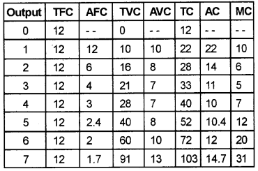
From the table given below
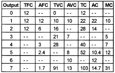
- Fill the blank columns
- Using the information in the table draw TC, TVC, TFC in one and AC, AVC, AFC, MC in other and prepare a short note on them.
Answer:
1.
2. Use the data to draw the diagram.
TC, TVC and TFC represent total costs. TC = TFC + TVC. TFC is the cost incurred on fixed factors. TVC is the cost incurred on variable costs. Even though the level of output is zero there will be some costs. This is known as fixed cost. When the level of output is zero total variable costs also will be zero.
It will increase as the level of output increases. AFC is the cost that always falls. It is a rectangular hyperbola. AVC, AC, MC are ‘U’ shaped. The MC will always pass through the minimum oftheAVCand AC.
