Kerala Plus Two Computerized Accounting Practical Question Paper March 2019 with Answers
| Board | SCERT |
| Class | Plus Two |
| Subject | Accountancy |
| Category | Plus Two Previous Year Question Papers Answers |
Time Allowed: 2 hours
Cool off time: 15 Minutes
Maximum Marks: 40
General Instructions to Candidates:
- There is a ‘cool off time’ of 15 minutes in addition to the writing time of 2 hrs.
- You are not allowed to write your answers nor to discuss anything with others during the ‘cool off time’.
- Use the ‘cool off time’ to get familiar with the questions and to plan your answers.
- Read questions carefully before you answering.
- All questions are compulsory and only internal choice is allowed.
- When you select a question, all the sub-questions must be answered from the same question itself.
- Calculations, figures and graphs should be shown in the answer sheet itself.
- Malayalam version of the questions is also provided.
- Give equations wherever necessary.
- Electronic devices except non-programmable calculators are not allowed in the Examination Hall.
Part – A
(Attempt any two questions, 2 × 6 = 12)
Question 1.
Given below is a table showing the name, Designation and Monthly salary paid for different employees in Babu Agencies for March 2018.
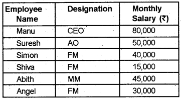
Find out the following
a) Total monthly salary by naming the concerned range as Total-Salary.
b) The total monthly salary paid to the Finance Manager (FM) in the firm.
c) The name of employee with monthly salary ₹ 40,000 by using LOOKUP Function.
Answer:
1. Procedure
Step 1 – Open Libre Office Calc Worksheet
Applications → Office LibreOffice Calc
Step 2 – Enter the data in the appropriate cells.

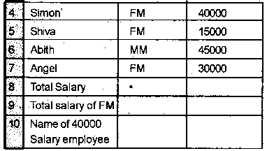
Step 3 – Naming a range
Select the range C2 : C7, click on “Data” from the menu bar. select “Define Range”. Type the name “TOTAL-SALARY in the name box and press OK or Enter key.
Step 4 – Enter the following formulas in respective cells.
| B8 | = SUM (TOTAL-SALARY) |
| B9 | = SUM IF (B2:B7 “FM” C2:C7) |
| B10 | = LOOK UP (40000, C2:C7, A2:A7) |
Output:
| (a) | 2,60,000 |
| (b) | 85,000 |
| (c) | SIMON |
Question 2.
Shinu obtained the following scores out of 100 in his higher secondary examination, March 2017.
| Subjects | Scores |
| English | 85 |
| Malayalam | 96 |
| Business Studies | 76 |
| Accountancy | 67 |
| Economics | 29 |
| Computer Application | 45 |
Convert the above scores into grades for each subject based on the following criteria by using IF function.
Scores Grade
| Scores | Grade |
| 90 – 100 | A+ |
| 80 – 89 | A |
| 70 – 79 | B+ |
| 60 – 69 | B |
| 50 – 59 | C+ |
| 40 – 49 | C |
| 30 – 39 | D+ |
| 20 – 29 | D |
| Below 20 | E |
Answer:
Procedure:
Step 1 – Open Libre Office Calc Worksheet
Applications → Office → LibreOffice Calc
Step 2 – Enter the data in the given cells.
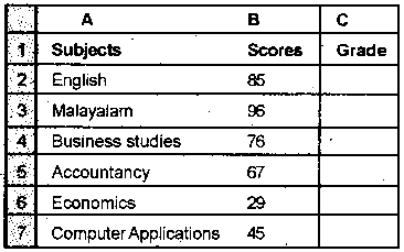
step 3 – Enter the following formula in C2
= IF (B2> =90, “A+”, IF (B2>=80, “A”, IF (82> =70, “B+”, IF (B2> = 60, “B”, IF (B2>=50, “C+”, IF (B2>= 40, “C”, IF(B2 > = 30, “D+”, IF(B2 > = 20, “D”, “E”))))))))
Step 4 – Drag and copy the formula up to C7
Output:
| Subjects | Grade |
| English | A |
| Malayalam | A+ |
| Business Studies | B+ |
| Accountancy | B |
| Economics | D |
| Computer Application | C |
Question 3.
Consider the following table

Answer the following questions using appropriate functions.
a) How many cells contain Numbers only?
b) Count the Number of cells contain any value?
c) Count the Number of cells containing the value exceeding 1000.
Answer:
Procedure:
Step 1 – Open Libre Office Calc Spreadsheet
Applications → Office → LibreOffice Calc
Step 2 – Enter the Table in the given range

Step 3 – Enter the given details and formula in the following cells

Output:
| (a) | 12 |
| (b) | 18 |
| (c) | 2 |
Question 4.
From the following information create a Pivot Table to give country wise sales of the
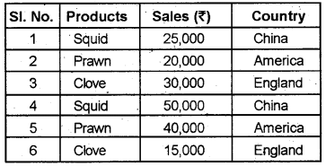
Answer:
Procedure:
Step 1 – Open Libre office Calc Spreadsheet
Applications → Office → LibreOffice Calc
Step 2 – Enter the data in the given cells.
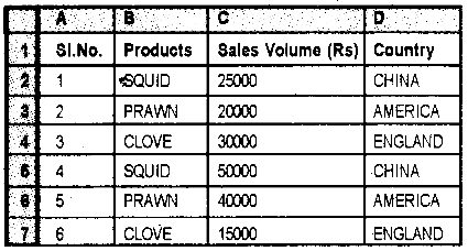
Step 3 – Select the range A1:D7 to create a Pivot Table. Then go to “Data” from the menu bar. Select “Pivot Table” click on “Create”
Data → Pivot Table → Create
Step 4 – A “Select Source” Window appears, Here select “Current Selection” and click “OK” button.
Step 5 – In the “Pivot Table Layout” window drag fields for the Pivot Table from the “Available Fields” as follows
Products ⇒ Row fields
Country ⇒ Column fields
Sales voulme ⇒ Data fields
and click on OK button
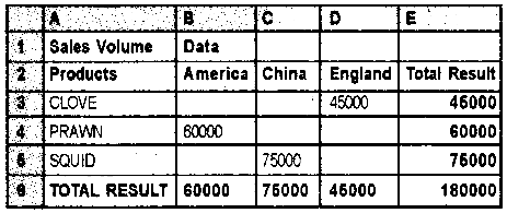
Question 5.
Mr. Biju intends to apply for Civil Service Examination this year. But the upper age limit is 32 as on 01.08.2018. Determine whether he is eligible to apply or not based on the cut off age. His date of birth is 06.09.1984. Use appropriate spreadsheet functions.
Answer:
Procedure:
Step 1 – Open Libre Office Calc Worksheet
Applications → Office → LibreOffice Calc
Step 2 – Enter the following details and formula in appropriate cells.
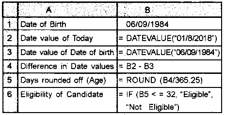
Output:
| Age | |
| Eligibility | Not Eligible |
Question 6.
A) Following are the scores obtained by some students in a competitive examination. Find out the Highest, Lowest and Average scores using appropriate function in spread sheet.

B) From the data given below fill the address in F2 using CONCATENATE FUNCTION.

Answer:
A) Procedure:
Step 1 – Open Libre Office Calc Spreadsheet
Applications → Office → LibreOffice Calc
Step 2 – Enter the formula and Other details in the given cells.

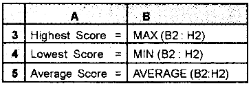
Output:
| (a) | 515 |
| (b) | 150 |
| (c) | 308 |
A) Procedure
Step 1 – Open Libre Office Calc Spreadsheet
Applications → Office → LibreOffice Calc
Step 2 – Enter the details in the following cells.

Step 3 – Enter the following formula in F2 cell.
= CONCATENATE (A2, “,”, B2, “,”, C2, “,”, D2, “,”, E2)
Output:
Jaya, Deepam, New street, Kozhikode, 680534
Question 7.
A) From the following table find out the Basic Pay of Mr. Ajith using VLOOKUP Function using EMPCODE 1846
| Emp. code | Name | Basic Pay |
| 1512 | Vinu | 7,000 |
| 3475 | Akhil | 11,500 |
| 1846 | Ajith | 8,500 |
| 5432 | Sonu | 6,000 |
B) From the following details, find out the actual profit for QUARTER II using VLOOKUP Function.

Answer:
Procedure:
Step 1 – Open Libre Office Calc Spreadsheet
Applications → Office → LibreOffice Calc
Step 2 – Enter the given details in appropriate cells.
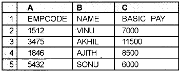
Step 3 – Enter the given details and formula in the following cells.
| A | B | |
| 6 | Basic Pay of Ajith | = VLOOKUP(1846, A2:C5, 3, 0) |
Output:
₹ 8500
B) Procedure:
Step 1 – Open Libre Office Calc Spreadsheet
Applications → Office → LibreOffice Calc
Step 2 – Enter the details in appropriate cells.

Step 3 – Enter the given formula and details in the following cells.
| A | B | |
| 5 | Profit for Quarter II | = HLOOKUP (C1, B1: E4, 4, 0) |
Output:
![]()
Question 8.
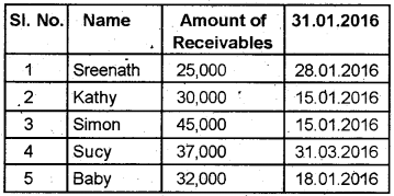
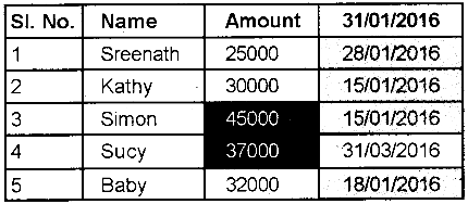
List of Debtors and the amount dues from them are given below. Apply conditional formatting to highlight receivables with date that have expired on 31.01.2016. Also hightlight the receivables more than ₹ 35,000 with red colour.
Answer:
Procedure:
Step 1 – Open Libre Office Calc Worksheet
Applications → Office → LibreOffice Calc
Step 2 – Enter the given details in the following cells.
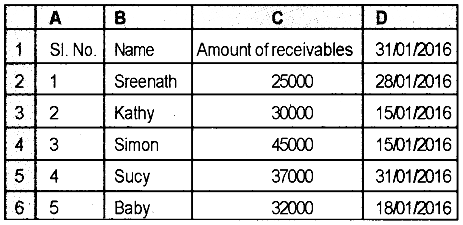
Step 3 – (1) To highlight receivables with date that have expired on 31/01/2016.
Select the range D2:D6 → Go to Format → Click on Conditional formating → Condition → select cell value is less than → Click on the next field and select cell D1 → in apply style, select new style from the drop down menu and click on Background and select Green colour → click on OK button click on OK button.
(2) To highlight receivables more than 35000
Select range C2:C6 → Go to Format → click on Conditional formating → Condition → select Cell value is greater than → click on the next field and enter the value 35000 → in apply style, select new style from the drop down menu and click on Background and select Red colour → click on OK button → click on OK button → click on OK button.
output:
Question 9.
Consider the following information
Loan Amount – ₹ 3,00,000
No. of Payments – 48 months
Annual Rate of Interest – 10%
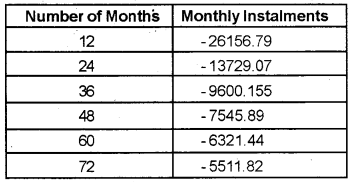
Prepare a one variable table showing the repayment of the above loan indifferent number of payment such as 12 months, 24 months, 36 months, 48 months, 60 months and 72 months. Use PMT Function.
Answer:
Procedure:
Step 1 – Open a new blank Worksheet in LibreOffice Calc
Applications → Office → LibreOffice Calc
Step 2 -Enter the following details in appropriate cells.
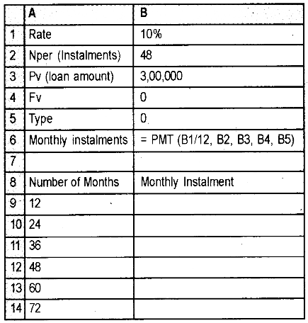
Step 3 – Select the range A8 : B13 and click on “Data” and select “Multiple Operations”.
Enter given details in Multiple Opeation
Windo
Formulas : 6
Row input cell : Leave it blank
Column input cell : 2
Press OK button
Output:
Part – B
(Attempt any Two questions, 2 × 4 = 8)
Question 10.
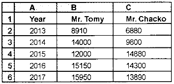
The total commission earned by Mr. Tomy and Mr. Chacko for the year 2013 – 2017 are given below.
| Year | Mr. Tomy | Mr. Chacko |
| 2013 | 8,910 | 6,880 |
| 2014 | 14,000 | 9,800 |
| 2015 | 12,000 | 14,880 |
| 2016 | 15,150 | 14,300 |
| 2017 | 15,950 | 13,890 |
a) Present the data in a Column Chart.
b) Change the chart type to Line Chart.
Answer:
a) Procedure:
Step 1 – Open Libre Office Calc Worksheet
Applications → Office → LibreOffice Calc
Step 2 – Enter the given table as follows.
Step 3 – Select the range A1:C6
Step 4 – Click on Insert menu → click on Chart → Chart wizard → click on Column chart → click 2D look → select Bar Chart → Finish.
Output:
വരയ്ക്കണം)
(b)
Step 5 – To change the chart type → click on the Chart Area → Format → Chart Type → select Line chart → OK
Out Put:
വരയ്ക്കണം
Question 11.
Draw a Pie Chart for the following data on vehicles registered in the motor vehicles department during 2016 – 2017 in a city.

Answer:
Step 1 – Open Libre Office Calc Worksheet
Applications → Office → LibreOffice Calc
Step 2 – Enter the data in respective cells.
| A | B | |
| 1 | Vehicle Type | Number of Vehicles |
| 2 | Bus | 575 |
| 3 | Truck | 5889 |
| 4 | Auto Rickshaw | 12345 |
| 5 | Car | 9765 |
| 6 | Two Wheeler | 23456 |
| 7 | Heavy Vehicles | 65 |
Step 3 – Select the range A2 : B7
Step 4 – Click on Insert menu → click on chart → chart wizard → from chart type, click on Pie Chart → Next → Next → Next → In chart Elements, give the title “vehicles registered in 2016 – 17” → Finish
Output:
വരയ്ക്കണം
Question 12.
Draw a column chart for the following data.

Answer:
Procedure:
Step 1 – Open a Libre Office Calc Spreadsheet
Applications → Office → LibreOffice Calc
Step 2 – Enter the following data in appropriate cells.
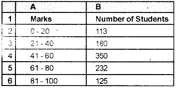
Step 3 -Select the range A2:B6 which is to be shown in the chart.
Step 4 – Click on Insert menu → click on Chart → Chart wizard → from chart type, click on Column Chart → Next → Next → Next → In Chart Elements, give the following
Title : Result
X axis : Marks
Y axis : Number of students
Then click on Finish
Output:
വരയ്ക്കണം
Question 13.
Below are the details of various assets in a firm.
Calculate depreciation under Straight Line Method using spreadsheet software.

Answer:
Procedure:
Step 1 – Open a new blank Worksheet in LibreOffice Calc.
Applications → Office → LibreOffice Calc
Step 2 – Enter the following data formula in the following way.
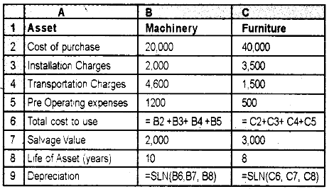
Output:
| Depreciation | |
| Machinery | 2580.00 |
| Furniture | 5312.50 |
Question 14.
BBC Ltd. purchased a machine on 01.01.2018 for ₹ 2,00,000 apd spend ₹ 10,000 for the installation. The machinery was installed on 10.01.2018. The expected salvage value is ₹ 8,000 at the end of its useful life of 10 years. Calculate annual depreciation under SLIM method using spreadsheet.
Answer:
Procedure:
Step 1 – Open a new blank Worksheet in LibreOffice Calc.
Applications → Office → LibreOffice Calc
Step 2 – Enter the given details in appropriate cells.
| A | B | |
| 1 | Name of Asset | Machine |
| 2 | Cost of purchase | 2,00,000 |
| 3 | installation Charges | 10,000 |
| 4 | Total cost to use | = B2 + B3 |
| 5 | Salvage value | 8000 |
| 6 | Life of Asset (years) | 10 |
| 7 | Depreciation | = SLNSLN(B4, B5, B6) |
Output:
![]()
Question 15.
A machinery was purchased on 1st April 2014 for ₹ 2,00,000. Its estimated life is 10 years with Slavage value of ₹ 20,000. Accounting year is 1st April to 31st March every year. Using built in function (spreadsheet), calculate depreciation under the Diminishing Balance Value method for 5 years.
Answer:
Procedure:
Step 1 – Open a new Spreadsheet in Libre Office Calc.
Applications → Office → LibreOffice Calc
Step 2 – Enter the given details as follows cells.
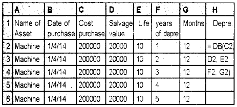
Step 3 – Drag the equation entered in H2 to H6
Output:
| Year of Depreciation | Amount of depreciation |
| 1 | ₹ 41,200.00 |
| 2 | ₹ 32,712.80 |
| 3 | ₹ 25,973.96 |
| 4 | ₹ 20,623.33 |
| 5 | ₹ 16,374.92 |
Question 16.
The following are the details of a plant and machinery. Calculate depreciation under WDV method using spreadsheet.
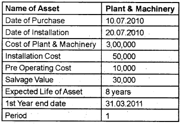
Answer:
Procedure:
Step 1 – Open a new Spreadsheet in Libre Office Calc.
Applications → Office → LibreOffice Calc
Step 2 – Enter the given details as follows.

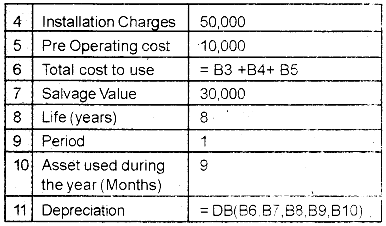
Output:
![]()
Question 17.
Prepare a Payroll of the following employees
| Name | Basic Pay | PF Loan |
| Sindhu | 39,500 | 11,100 |
| Ashly | 41,500 | 11,800 |
| Unni | 41,500 | 11,300 |
| Ranjith | 54,000 | 0 |
| Bindu | 48,000 | 11,700 |
| Ambily | 48,000 | 11,850 |
| James | 41,500 | 12,000 |
| Thara | 62,000 | 0 |
| Arun | 33,500 | 12,000 |
| Rahim | 38,000 | 5,500 |
Additional information
1. DA – 30% of Basic Pay
2. HRA – ₹ 1,500 for employees Basic Pay greater than ₹ 52,000, for others ₹ 1,300
3. TA – ₹ 500 per employee
4. PF Subscription – 6% for Gross Pay
5. TDS – 20% for Gross Pay greater than ₹ 60,000, otherwise 10%
Answer:
Procedure:
Step 1 – Open a new Spreadsheet in LibreOffice Calc.
Applications → Office → LibreOffice Calc
Step 2 – Enter the following text/formula in respective cells.
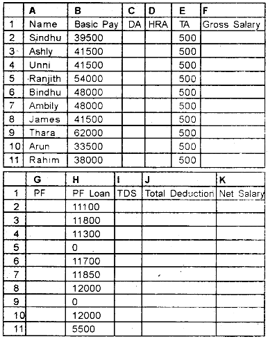
Step 3 – Enter the given details
| Cell | Formula |
| C2 | = B2 * 30% |
| D2 | = IF (B2>52000, 1500, 1300) |
| F2 | = Sum (B2:E2) |
| G2 | = F2 * 6% |
| 12 | = IF (F2>60000, F2 * 20%, F2 * 10%) |
| J2 | = Sum (G2 :I2) |
| K2 | = F2 – J2 |
Step 4 – Copy the formula upto the last employee.
Output:
| Name | Net Salary |
| Sindhu | 33546 |
| Ashly | 35030 |
| Unni | 35530 |
| Ranjith | 53428 |
| Bindhu | 35808 |
| Ambily | 35658 |
| James | 34830 |
| Thara | 61124 |
| Arun | 26094 |
| Rahim | 37508 |
Question 18.
Mr. Binu has taken a loan of ₹ 6,00,000 from a bank, interest @10% per annum. The loan is repayable over a period of 10 years in monthly instalments. Prepare a loan repayment schedule by showing outstanding balance for the first year. (Hint: Use PMT Function)
Answer:
Procedure:
Step 1 – Open a Libre Office Calc new Worksheet.
Applications → Office → LibreOffice Calc
Step 2 – Enter the data/formula as follows,
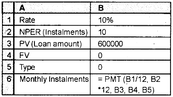
Output:
![]()
Part – C
(Attempt One question, (1 × 6 = 6)
Question 19.
The various transactions relating to Modern Pharma for the month of January 2018 is given below. Ascertain cash balance for the month using an accounting software
Jan. 1 – Started business with cash ₹ 60,000
Jan. 1 – Purchased office furniture ₹ 4,500
Jan. 1 – Cash purchases ₹ 20,000
Jan. 1 – Credit sales to Anu ₹ 40,000
Jan. 2 – Salary to staffs ₹ 10,000
Jan. 2 – Received from Anu ₹ 18,000
Answer:
Procedure:
Step 1 – Open GNUKhata:
Applications → Office → GNUKhata:
Step 2 – Create Organisation
Create a new organisation Modern Pharmacy – Profit making – 01/01/2018 to 31/12/18
Step 3 – Create Admin and Login:
Supply adequate information – username, password, security question & answer.
Step 4 – Create Ledger Accounts:-
Supply adequate information – using the Analysis Table given below.
Master Menu → Create Account
(Leave blank opening balance column while creating ledger accounts)
Analysis Table
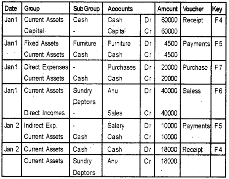
Step 5 – Voucher Entry
Select the appropriate voucher form Voucher menu – Enter number and date – select Debit, Enter amount – select Credit, enter amount – Save
Transaction → Select Appropriate Voucher
Step 6 – Display Cash book
Report → Ledger → select Cash Account → View
Output:
![]()
Question 20.
Enter the following transactions by using suitable accounting vouchers and display the Profit & Loss Account and Balance Sheet.
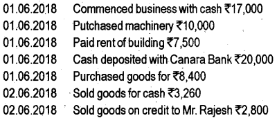
Answer:
Procedure:
Step 1 – Open GNUKhata:-
Applications → Office → GNUKhata:
Step 2 – Create Organisation
Create a new organisation – Profit making – with imaginary data
Step 3 – Create Admin and Login:
Supply adequate information – username, password,
Step4 – Create Ledger Accounts:-
Supply adequate information – using Analysis Table given below.
Master Menu → Create Account
(Leave blank the opening balance column while creating ledger accounts)
Analysis Table
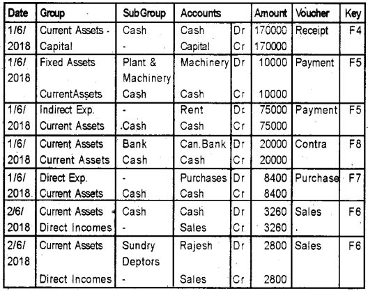
Step 5 – Voucher Entry:-
Select appropriate voucher from Voucher menu – Enter number and date – select Debit, Enter the amount – select Credit, enter the amount – Save
Transaction → Select Appropriate Voucher
Step 6 – Display Profit and Loss Account:
Report → Profit & Loss → view
Step 7 – Display Balance Sheet
Balance Sheet
Report → Balance sheet → view
Output:
| Profit & Loss Account – Net Loss | 9840 |
| Balance sheet Total | 160160 |
Question 21.
Create the following ledgers in an accounting software and display the Balance Sheet as on 31.12.2018
| Items | Amount |
| Capital | 2,50,000 |
| Loose Tools | 50,000 |
| Creditors | 50,000 |
| Bank Loan | 75,000 |
| Land and building | 1,00,000 |
| Plant and Machinery | 73,000 |
| Motor Vehicle | 75,000 |
| Debtors | 50,000 |
| Outstanding Salary | 3,000 |
| Cash in hand | 30,000 |
Answer:
Procedure:
Step 1 – Open GNUKhata:-
Applications → Office → GNUKhata:
Step 2 – Create Organisation
Create a new organisation – Profit making – with imaginary data
Step 3 – Create Admin and Login :-
Supply adequate information – username, password,
Step 4 – Create Ledger Accounts:-
Supply adequate information – using Analysis Table given below.
Master Menu → Create Account
(Leave blank the opening balance column while creating ledger accounts).
Analysis Table (Trial Balance)
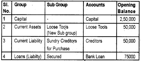
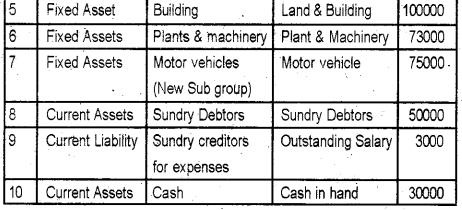
Step – 5 – Display Balance Sheet
Report → Balance sheet
Output:
![]()
Part – D
(Attempt One question, 1 × 6 = 6)
Question 22.
Enter the following in a database table with the file name Emp_details.
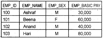
a) Display the name of employees drawing BASICPAY greater than or equal to 60,000
b) Display the name of employees begin with A’.
Answer:
Procedure:
Step 1 – Libre Office Base
Applications → Office → LibreOffice Base
Step 2 – Create a new Data base
Data base wizard → Create New Data base → Next → Yes, register database for me → open the database for editing → Finish
Step 3 – Save New database
In save dialogue box, give the name Emp -Details and select the location to save the database and click save button.
Step 4 – Create a database Table
Database Pane → Tables → Create Tables in Design veiw
Step 5 – Field Name Entry
In Table Creation screen, enter the Field Names and select appropriate Data Types as given below.
| Field Name | Field Type/Data Type |
| emp_id | Number |
| emp_name | Text |
| emp_sex | Text |
| emp_basic pay | Number |
Step 6 – Setting Primary key
To set emp-id as Primary Key, Right click → select Primary key from the drop down menu.
Step 7 – Save Table
Click on File → Select Save button → In Save as dialogue box, Enter TBLEMP as the name and click on OK button → Close the Table creation screen.
Step 8 – Data Entry
Data base pane → Tables → Created Tables
Select TBLEMP → Doubleclick to open it.
Enter all data one by one and save the table.
Step 9 – Create Query
a) From Database pane, click on Queries button and in the right side under Tasks section, click on create query in Design View. Now Add Table or Query window opens.
b) Select the table TBLEMP and click Add button, then close the window
c) In the Query Design Window, double click, on each Field in Table window to add all the fields to query design grid.
Step 10 – Enter Query Criteria (Question 1)
a) In the Query Design Grid, set the criteria for the query. Enter >=60000 in the criterion row in emp_basic pay
b) Click on the Run Query button or press F5 to display the result.
c) Save and close the Query
File → Save “Save as” window opens, give the name
Query 1 and click on OK button.
Step 11 – Enter Query Criteria (Question 2)
a) In the Query Design Grid, set the criteria for the query. Enter like ‘A*’ in the criterion raw in emp_name column.
b) Click on the Run Query button or press F5 to display the result.
c) Save and close the Query
File → Save “Save as” window opens, give the name
output – 1

output – 2

Question 23.
Create a database table named TABLE_EMPLOYEE and enter the following details using a form

Also create a query to display EMP_NAME and BP.
Answer:
Procedure:
Step 1 – Open Libre Office Base
Applications → Office → LibreOffice Base
Step 2 – Create a new Data base
Database wizard → Create New Database → Next → Yes, register data base for me → open database for editing → Finish
Step 3 – Save New database
In save dialogue box, give the name Emp – Details and select the location to save the database and click save button
Step 4 – Create a database Table
Data base Pane → Tables → Create Tables in Design veiw
Step 5: Field Name Entry
In Table Creation screen, enter the Field Names and select appropriate Data Types as given below.
| Field Name | Field Type/Data Type |
| Emp_id | Number |
| emp_name | Text |
| emp_bp | Text |
| empjira | Text |
Step – 6 Setting Primary key
To set emp_id as Primary Key, Right click → select Primary key from the drop down menu.
Step 7 – Save Table
Click on File → Select Save button → In Save as dialogue box, Enter TBLEMP as the name and click on OK button → Close the Table creation screen.
Step 8 – Data Entry
Database pane → Tables → Created Tables
Select TBLEMP → Double click to open it.
Enter all data one by one and save the table.
Step 9 – Create Query
a) From Data base pane, click on Queries button and in the right side under Tasks section, click on create query in Design View. Now Add Table or Query window opens.
b) Select the table TBLEMP and click Add button, then close the window
c) In the Query Design Window, double dick, on emp_name field and emp_bp field to add to query design grid
Step 10 – a) Click on Run Query button or press F5 to display the result.
b) Save and close query File → Save. “Save as” window opens, give name Query 1 and click on OK button.
Output:
| Query | |
| emp_ name | emp_bp |
| Sajith | 20,000 |
| Suresh | 30,000 |
| Anil | 40,000 |
Question 24.
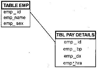
Create a data base table named EMPLOYEE and PAY_DETAILSwiththefollowing filed:

Create relationship between theses two tables.
Answer:
Procedure:
Step 1 – Libre Office Base
Applications → Office → LibreOffice Base
Step 2 – Create a new Data base
Database wizard → Create New Data base → Next → Yes, register data base for me → open the database for editing → Finish
Step 3 – Save New database
In save dialogue box, give the name Emp. Details and select the location to save the database and click save button.
Step 4 – Create a database Table
Data base Pane → Tables → Create Tables in Design veiw
Step 5 – Field Name Entry
In Table Creation screen enter, the Field Names and select appropriate Data Types as given below

Step – 6 Setting Primary key
To set emp_id as Primary Key, Right click → select Primary key from the drop down menu.
Step 7 – Save Table
Click on File → Select Save button → In Save as dialogue box, Enter TBLEMP as the name and click on OK button → Close the Table creation screen.
Step 8 – Data Entry
Database pane → Tables → Created Tables
Select TBLEMP → Double click to open it.
Enter all data one by one and save the table
Step 9 – In the same way create another table – TBL PAY_ DETAILS with the following fields.
Step 10 – Create Relationship
a) Tools → Relationship
From Add Tables window, Add TBLEMP and TBLPAYDETAILS. Then Click on close button. Then Click on, Save button.
b) In the relationship window, click on emp_id feild of TBLEMP table and drag and drop on to emp_id field of TBLPAYDETAILS table. Then a Relationship line between these two tables is formed.
Output:
