Kerala Plus Two Computerised Accounting Chapter Wise Questions and Answers Chapter 2 Spread Sheet
Plus Two Accountancy Spread Sheet One Mark Questions and Answers
Question 1.
The best way to get started in Libre Office calc is _____
Answer:
Application → Office → LibreOffice Calc
Question 2.
___________ is a configuration of rows and columns
Answer:
Spread sheet
Question 3.
A spread sheet is also known as ____________
(a) Work book
(b) Work area
(c) Work sheet
(d) Spread book
Answer:
(c) Work sheet
Question 4.
____________ in spread sheet are horizontal vectors while ______ are vertical vectors
Answer:
Rows, columns
Question 5.
Spread sheet is used to
(a) Record data
(b) Calculate data
(c) Compare data
(d) All the above
Answer:
(d) All of the above
Question 6.
Each cell value can either be an independent (basic) value or it may be derived on the basis of ____________.
Answer:
Arithmetic expression or a function.
Question 7.
A file in LibreOffice Calc is known as a ______
(a) Work sheet
(b) Page
(c) Work book
(d) All the above
Answer:
(c) Workbook
Question 8.
A workbook is a collection of a number of ______
Answer:
Work Sheets
Question 9.
Where is the address of the active cell displayed?
(a) Row heading
(b) Status Bar
(c) Name Box
(d) Formula Bar
Answer:
(c) Name Box
Question 10.
Which command reverses the last action performed in the worksheet?
(a) Cut
(b) Undo
(c) Redo
(d) Paste
Answer:
(b) Undo
Question 11.
__________ is a text or special character or descriptive information for rows or columns.
Answer:
Label
Question 12.
A formula must starts with a ___________ sign
(a) =
(b) >
(c) *
(d) {}
Answer:
(a) =
Question 13.
_______ Function is commonly used to get the addition of various numbers orthe contents of various cells.
Answer:
Autosum (Σ)
Question 14.
The cell A5 indicate Column _______ and Row _____
Answer:
Column A & Row 5
Question 15.
The dark box which distinguishes the active cell is called _______
Answer:
Cell Pointer
Question 16.
One or more cells selected is called ______
Answer:
a range
Question 17.
Without the equal sign, the entry in a cell is treated as _________
(a) Text
(b) Label
(c) TextorLabel
(d) None of the above
Answer:
(c) Text or Label
Question 18.
Libre Office calc has three type of cell entries, they are _______ , ______and _______
Answer:
Value, Label and Formula.
Question 19.
Which command allows you to reverse an undo command?
(a) Redo
(b) Repeat
(c) Reset
(d) Reverse
Answer:
(a) Redo
Question 20.
Which cell alignment is assigned to most values by default?
(a) Right
(b) Left
(c) Centre
(d) None of the above
Answer:
(b) Left
Question 21.
Which function automatically totals a column or row of Values?
(a) TOTAL
(b) ADD
(c) SUM
(d) AVG
Answer:
(c) SUM
Question 22.
Which Mathematical Operator is represented by an asterisk (*)
(a) Exponentiation (square)
(b) Addition
(c) Subtraction
(d) Multiplication
Answer:
(d) Multiplication
Question 23.
How many blank work sheets are shown when a new workbook is created?
(a) One
(b) Two
(c) Three
(d) Four
Answer:
(c) Three
Question 24.
The cell co-ordinate in the formula are known as ………….
Answer:
cell references
Question 25.
IF function is …………….
Answer:
Logical function
Question 26.
The cell references for cell range of G2to M12 is …………….
(a) G2.M12
(b) G2: M12
(c) G2; M12
(d) G2 – M12
Answer:
(c) G2: M12
Question 27.
If 4/6 entered in a cell without applying any format, LibreOffice Calc will treat this as
(a) Fraction
(b) Number
(c) Text
(d) Date
Answer:
(d) Date
Question 28.
The cell labelled F5 refers to …………….
(a) Row F column 5
(b) Column F row 5
(c) Function available in cells
(d) Function key F5
Answer:
(b) Column F row 5
Question 29.
LibreOffice Calc is a FOSS. What is FOSS?
Answer:
Free and Open Source Software.
Question 30.
Which among the following is not a spreadsheet software.
(a) MS Office Excel
(b) Open Office Spredsheet
(c) Libre Office Calc
(d) MS Office Word
Answer:
(d) M S Office Word
Question 31.
How many worksheets can be made as active worksheet at a time?
(a) 1
(b) 2
(c) 3
(d) 4
Answer:
(a) 1
Question 32.
The name of the worksheet will be shown in the ______ at the bottom left of the windows.
Answer:
Sheet Tab
Question 33.
To add column in a worksheet, click __________, there we get an option to add column.
Answer:
Column Header
Question 34.
A ………… is identified by a combination of a column header (letter) and a row header (number)
Answer:
cell
Question 35.
_______ is a group of adjacent cells that forms a rectangular area.
Answer:
Range
Question 36.
Which among the following is used as the range operator
(a) ;
(b) :
(c) /
(d) #
Answer:
(b) :
Question 37.
One ENTER key stroke means
(a) One cell down
(b) One cell up
(c) One cell right
(d) One cell left
Answer:
(a) One cell down
Question 38.
………………. Function counts the number of cells which contain any value.
(COUNT, COUNTA, COUNT BLANK, COUNTIF)
Answer:
COUNTA
Plus Two Accountancy Spread Sheet Two Mark Questions and Answers
Question 1.
Match the following
| A | B |
| 1. Rows | 1. Intersection of a row & a column |
| 2. Columns | 2. Numerical numbers from top to bottom |
| 3. Cell | 3. Unique identification code of a cell |
| 4. Cell address | 4. Alpha characters from left to right |
Answer:
| A | B |
| 1. Rows | 1. Numerical numbers from top to bottom |
| 2. Columns | 2. Alpha characters from left to right |
| 3. Cell | 3. Intersection of a row & a column |
| 4. Cell address | 4. Unique identification code of a cell |
Question 2.
What do you mean by spreadsheet?
Answer:
Spreadsheet:
Spreadsheet application is a computer program that allows to record, calculate and compare numerical or financial data. Using a spreadsheet program. We can store a lot of data in the worksheet and also arrange and analyse the data by using different functions and formulae for the meaningful object.
It is used to establish relationship between two or more sets of data. Libre Office Calc, MS Office Excel, Open Office Spreadsheet etc. are examples of spreadsheet software.
Question 3.
Give a short note on
- Work book
- Work sheet
Answer:
1. Workbook:
A file in spread sheet is known as a workbook. A work book is a collection of a number of work sheets.
2. Work sheets:
The work area which consists of rows and columns in a spreadsheet is called a worksheet. By default three work sheets-sheet 1, sheet -2, sheet -3 are available in work book.
Question 4.
Explain about rows and columns in Libre Office Calc?
Answer:
1. Rows:
Rows are the horizontal vectors in the worksheet. These are numbered numerically from Top to Bottom.
2. Columns:
Columns are vertical vectors in the worksheet. These are referred by alpha characters from left to right such as A, B, C, …, AA, AB, AC …etc.
Question 5.
What do you mean be Relative cell Reference?
Answer:
1. Relative Cell references:
By default cell reference is relative; which means that as a formula or function is copied and pasted to other cells, the cell references in the formula or function change to reflect the new location.
Question 6.
Define the following
- Label
- Formula
Answer:
1. Labels:
Descriptive information for rows or columns in the form of a text or a special character is called Label.
Eg: Name, Roll No, Address.
2. Formula:
The formula means a mathematical calculation on a set of cells. The formula must start with an = (equal to) sign. When a cell contains a formula, it often contains reference to other cells. Eg:= Basic pay + DA + HRA
Question 7.
List down any two features fo Spreadsheet.
Answer:
- A spreadsheet is a configuration of rows and columns.
- A spreadsheet is also known as worksheet.
Question 8.
Name the different spreadsheet software available.
Answer:
LibreOffice Calc, MS Office Excel, Open Office Spreadsheet.
Question 9.
Briefly explain any two Date and Time functions availabe in LibreOffice Calc
Answer:
1. TODAY():
It is the function for today’s date in the worksheet. This helps to update the date value when we reopen the spreadsheet or modify the values of the document
Syntax: =TODAY()
2. NOW ():
It is the function for today’s date and present time. This helps to update the date and the time value when the cell value is modified.
Syntax: =NOW()
Question 10.
Give the Syntax for
- YEAR()
- DATE()
Answer:
1. YEAR()
Syntax: = YEAR (Date value) OR = YEAR (“Date”)
2. DATE()
Syntax: = DATE (Year, Month, Day)
Question 11.
Complete the table by using ROUNDUP()
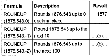
Answer:
- 1880
- 1900
Question 12.
What are the Text Manipulation Function in LibreOffice Calc
Answer:
- TEXT
- CONCATENATE
Question 13.
Give the explanation of the following errors
Error Message
- # DIV/o!
- VALUE!
Answer:
- # DIV/0! → When a number is divided by zero
- VALUE! → When a wrong argument is given in a fromula
Question 14.
Spot the correct pairs by observing the nature of software, and give justification
(a) Microsoft Excel and LibreOffice Calc
(b) Linux and Tata Ex.
(c) Windows and MS Office
(d) GINUGhata and Microsoft Access
Answer:
(a) Microsoft Excel and LibreOffice Calc. Both are spread sheet packages.
Plus Two Accountancy Spread Sheet Three Mark Questions and Answers
Question 1.
What are the advantage of Libre Office Calc?
Answer:
- It is both free software and open source software.
- It can be used to calculate, analyse and manage data.
- Libre Office Calc is available for a variety of platforms including Linux, OSX, Microsoft windows and Free BSD.
Question 2.
Give the cell address or range reference in the following situations.
- Cell at 10th column and 6th row.
- Cell at 27th column and 15th row.
- Range starting from 5th column, 9throw and spread till 12th column and 15th row.
Answer:
- Cell at 10th column and 6th row = J6.
- Cell at 27th column and 15th row = AA15.
- Range starting from 5th column, 9th row and spread till 12th column and 15th row = E9: L15.
Question 3.
- What is FOSS?
- What are the benefits of using FOSS?
Answer:
- FOSS means Free and Open Source Software
- The benefits of using FOSS:
- Decreased software costs.
- Increased Security and stability.
- Any one can use, copy, study and change the software in any manner.
- Source code is openly shared.
Question 4.
How can we save Libre Office Calc file?
Answer:
Step 1: Go to the File menu
File menu
Step 2: Click on Save
Save
OR
Step 1: & Step 2 – Press Ctrl + S
Ctrl + S
Step 3: Type the file in the name field instead of default name Untitled 1
Name field
Step 4: Choose the place where we want to save the new file.
Step 5: Click on Save
Question 5.
Write the steps to be followed to
- Rename a worksheet
- Delete a worksheet
- Copy a worksheet
Answer:
1. Rename a worksheet:
Step – 1 Select the work sheet in the Sheet Tab which we want to Rename.
Step – 2 Right click and select Rename sheet from the drop up menu
Step – 3 Type new name in the Name field and press OK button
2. Delete a worksheet:
Step – 1 Select the worksheet in the Sheet Tab which we want to delete
Step – 2 Right click and select Delete sheet from the drop up menu
Step – 3 Click on Yes to the conformation question.
3. Copy a worksheet:
Step – 1 Click on blank rectangle Top left corner of the worksheet (Range Adress A1: AM J1048576)
Step – 2 Move the curser inside the worksheet and Right click the mouse.
Step – 3 Click on Copy from the dropdown menu.
Step – 4 Open the worksheet where we want to copy the sheet
Step – 5 Right click on cell A1. Click on Paste.
Question 6.
Give the cell address or range reference in the following situations.
- Cell of 10th column and 9th row
- Range starting from 2nd column 4th row and spread till 8th column 12th row
- Range starting from 4th column 5th row and spread till 10thcolumn 15th row
Answer:
- J9
- B4: H12
- D5: J15
Question 7.
What is the purpose of the COUNTIF function?
Answer:
COUNTIF():
This function counts the number of cells within a given that meet the criteria or condition.
Syntax: = COUNTIF (Range, Criteria)
Question 8.
Write the command to calculate the State Life Insurance Premium (SLI) of an employee using IF Function. The condition is SLI Premium Rs. 500/-below Basic Pay (BP) of Rs. 15000/- and for others Rs. 800/- (BP is given in cell C3)
Answer:
= IF(C3 < 15000, 500, 800)
Question 9.
4 numbers are entered in Libre Office Calc spreadsheet starting from cell A1 to A4. Write any two formulae for getting total of those numbers in the cell A5
Answer:
- A5 = A1 + A2 + A3 + A4
- A5 = Σ(A1 : A4)
Question 10.
For preparation of Payslip of an employee, Govind entered Basic Pay in cell B2 of a worksheet in LibreOffice calc. The D.A. is 76% of Basic Pay and Gross Salary is the sum of Basic Pay and DA. In order to calculate the amount of DA in cell C2 and Gross salary in cell D2, what entries are to be made?
Answer:
Basic Pay → B2
DA → C2
Gross salary → D2
C2 = B2 * 76%
D2 = B2 + C2
Question 11.
Consider the following features of a software tool. Identify the software.
- It can be used as a text editor
- List out the important uses of this software
Answer:
- LibreOffice calc has the above mentioned features.
- Importance of LibreOffice calc.
- It can be used for the preparation of statement of depreciation.
- It can be used for preparation of Payroll of employees.
- It can be used for the preparation of the loan re-payment schedule.
Question 12.
Complete the following.
- One cell down → arrow key
- One cell up → …………………………
- One cell left → …………………………
- One cell right → ………………………
Answer:
2. Up arrow key
3. Left arrow key
4. Right arrow key
Question 13.
Can you give some key navigations and short cut in LibreOffice calc?
Answer:
Spreadsheet navigation:
We can move around a worksheet through four arrow keys
- Left-arrow key
- Right arrow key
- Up arrow key
- Down arrow key
The mouse can also be used for navigation in a spreadsheet except for data entry. Some common operations/navigations are listed below:
| Movement | Keystroke (Press Key) |
| One cell up | Up arrow key/ Shift + Enter key |
| One cell down | Down arrow key/ Enter key |
| One cell right | Right arrow key/ Tab key |
| One cell left | Left arrow key / Shift + Tab key |
| Top of sheet (Cell A1) | Ctrl + Home Key |
| Move to last cell containing data | Ctrl + End Key |
| Move to beginning of the Row | Home Key or Ctrl + Left arrow key |
| Move to last filled cell in column | End key |
Question 14.
What commands are used to insert a column and delete a column in LibreOffice Calc?
Answer:
1. To insert a column:
To insert a column click a cell in the column immediately to the right of where you want to insert the new column. Then on the Insert menu, click Columns.
2. To delete a column:
Select the column you want to delete. On the Edit menu, click Delete.
Question 15.
Give the procedure to insert a new worksheet and to delete a worksheet.
Answer:
To insert a new worksheet, right click the worksheet, select ‘insert’. To delete a worksheet, select the sheet you want to delete and ‘click delete sheet’ on the edit menu.
Question 16.
Give the cell address or range reference in the following situations.
- Cell at 12th Column and 8th row.
- Range starting from 6th Column 10th row and spread till 12th Column and 16th row.
Answer:
- L8.
- F10: L16
Question 17.
Name the appropriate Statistical functions.
- Number of cells contain numbers.
- Number of cells contain any value.
- Number of empty cell.
- Number of cells that meet the given criteria.
Answer:
- COUNT
- COUNTA
- COUNTBLANK
- COUNTIF
Question 18.
What is the use of financial function ACCRINT in LibreOffice Calc
Answer:
ACCRINT ():
This function returns the accrued interest for a security that pays periodic interest.
Syntax: = ACCRINT(Issue, First_Interest, settlement, rate, Par, frequency, basis, calc_method)
Question 19.
Explain the difference between relative cell reference and absolute cell reference?
Answer:
1. Relative Cell references:
By default cell reference is relative; which means that as a formula or function is copied and pasted to other cells, the cell references in the formula or function change to reflect the new location.
2. Absolute Cell reference:
The absolute cell reference consists of the column letter and row number surrounded by dollar ($) signs. Eg $A$5. An absolute cell reference is used when we want a cell reference to stay fixed on a specific cell.
Question 20.
What is the use of PIVOT TABLE?
Answer:
Preparation of reports using Pivot Tables:
A Pivot Table is a way to present information in a report format. A Pivot Table report provides enhanced layout, attractive and formatted report with improved readability. There are two types of data table.
- One-Variable Data Table (One – Variable )
- Two-Variable Data Table (Two-Variable)
- The one variable Data Table allows us to identify a single decision variable in our model and see how changing the values for that variable affects the values calculated by one or more formulas in our model.
- The two variable Data table allows us to specify two decision variables and a variety of inputs and only a single formula.
Plus Two Accountancy Spread Sheet Five Mark Questions and Answers
Question 1.
Define the following
- Cell
- Range
- Worksheet
- Workbook
Answer:
1. Cell:
The intersection of a row and a column is called a cell. A cell is identified by a combination of alpha – numeric character eg: A1, B6, C10, etc. This alphanumeric character is called cell address. Hence each cell has a unique address.
2. Ranges:
Range is a group of adjacent cells that forms a rectangular area. A range is specified by giving the address for first cell in range and the last cell in the rage, eg: range starting from A10 to A20 is written as A10: A20 where colon (:) is the range operator.
3. Worksheets:
The work area which consists of rows and columns in a spreadsheet is called worksheet. By default three worksheets-sheet 1, sheet -2, sheet -3 are available in the workbook.
4. Workbook:
A file in a spreadsheet is known as a workbook. A workbook is a collection of a number of worksheets.
Question 2.
What are the different spreadsheet reference functions in Libre Office Calc?
Answer:
Spreadsheet Reference Functions:
The important spreadsheet reference functions are
1. LOOKUP () functions:
The LOOKUP function returns a value either from a one-row or one-column range or from an array. The lookup function has two syntax forms: Vector form and Array form.
The vector form of LOOUP looks in a one-row or one-column range (known as a vector) for a value and then returns a value from the same position in a second one-row or one-column range.
The array form of LOOKUP looks in the first row or column of an array for the specified value and then returns a value from the same position in the last row or column of the array.
LOOKUP (Vector from)
Syntax: = LOOKUP (search criterion, Search vector, Result vector)
LOOKUP (Array form)
Syntax: =(LOOKUP (lookup_value, array)
2. VLOOK UP ():
VLOOK UP is the vertical LOOKUP function. Use VLOOK UP to search the first column (columns are vertical) of a block of data and return the value from another column in the same row.
Syntax: = VLOOKUP (Search criterion; Array; Index; Sort Order)
3. HLOOKUP ( ):
It is the Horizontal LOOKUP function, searches for a value in the first row of a table array and returns the corresponding value in the same column from another row of the same table array.
Syntax: HLOOKUP (search criteria; index; sorted)
Question 3.
Give the cell address or range reference in the following situations.
- Cell at 10th Column and 9th row.
- Range starting from 2nd Column 4th row and spread till 8th Column and 12th row.
Answer:
- J9.
- B4: H12
Question 4.
What are the logical functions in LibreOffice Calc
Answer:
Logical Functions:
Logical functions are used for comparison and checking a test condition. The major logical functions are IF, AND and OR.
Question 5.
Explain the steps involved to insert a new work sheet in LibreOffice Calc
Answer:
Steps involved to insert a new work sheet in LibreOffice Calc.
Step 1 – Click on the [+] button in the sheet Tab
OR
Step 1 – Click on the work sheet in the sheet Tab Sheet Tab
Step 2 – Right click the mouse
Step – 3 Select insert sheet from the Drop up menu box
Drop up
Step 4- Add number of sheets and give name, press
OK
Question 6.
You are required to prepare a rank list for admission to the B.Com course. The Index mark is calculated as follows.
Sum of mark secured in Plus 2, Mark obtained in Accountancy and -25% of Mark obtained in Business studies. Give the entries in Libre Office Calc to get the index mark.
Answer:
- A1 → Total Mark
- B1 → Mark in Accountancy
- C1 → Mark in Business Studies
- D1 → Index Mark
- A2 → Enter the Marks
- B2 → Enter the Marks
- C2 → Enter the Marks
- D2 → =A2 + B2 + (C2 * 25%)
Question 7.
Match the following:
| A | B |
| 1. One cell to the left | 1. Right arrow key |
| 2. To cell A1 | 2. Ctrl + End |
| 3. One cell to the right | 3. Ctrl + Home |
| 4. To the last cell in the worksheet that contains data | 4. Shift + Tab |
Answer:
| A | B |
| 1. One cell to the left | 1. Shift + Tab |
| 2. To cell A1 | 2. Ctrl + Home |
| 3. One cell to the right | 3. Right arrow key |
| 4. To the last cell in the work sheet that contains data | 4. Ctrl + End |
Question 8.
The monthly sales of a company for the first six months are given below:
| A | B |
| 1. January | 25000 |
| 2. February | 15000 |
| 3. March | 28000 |
| 4. April | 32000 |
| 5. May | 20000 |
| 6. June | 30000 |
- Find the total sales for the six months
- Find the average sales of the six months
- Find the lowest sales of the six months
- Find the highest sales of the six months
Answer:
| A | B |
| 7. Total sales | = SUM (B1:B6) |
| 8. Average sales | = Average (B1:B6) |
| 9. Lowest sales | = MIN (B1:B6) |
| 10. Highest sales | = MAX(B1:B6) |
Question 9.
Give the range reference in the following cases.
- Range beginning from 1st column, 1st row and ending 16th column, 8th row
- Range beginning from 5th column, 7th Row and ending 27th column, 37th row
Answer:
- A1: P8
- E7: AA37
Question 10.
Match the following:
| A | B |
| a) Today | a) Today’s date & Time |
| b) Now | b) Convert date into corresponding value |
| c) Day | c) Today’s date |
| d) Date value | d) Day of the data referred in the formula |
Answer:
| A | B |
| a) Today | a) Today’s date |
| b) Now | b) Today’s date & time |
| c) Day | c) Day of the date referred in the formula |
| d) Date value | d) Convert date into corresponding value |
Question 11.
Give the cell address or range reference in the following situations
- Cell at 8th column and 10th row
- Cell at 27th column and 6th row
- Range starting from 5th column, 9th row and spread till 12th column and 15th row
Answer:
- H10
- AA6
- E9: L15
Question 12.
What are the steps to be followed for naming cells and ranges.
Answer:
Step 1 – Select the cells or ranges that are to be named.
Step 2 – Select Define Range from the Data menu Data.
Step 3 – This will display a dialogue box us “Define Database Range”. It will provide a place to enter “Name”.
Step 4 – Click OK on the dialogue box.
Plus Two Accountancy Spread Sheet Practical Lab Work Questions and Answers
Question 1.
The following marks are obtained by 8 students in an examination.
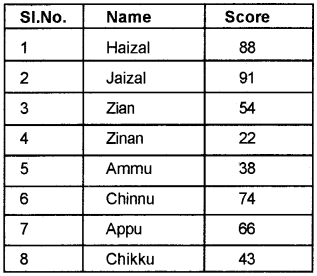
Ascertain the grade obtained by students based on the following criteria

Procedure:
Step 1 – Open Libre Office Cal work sheet
Applications → Office → Libre Office calc
Step 2 – Enter the data in the given cells
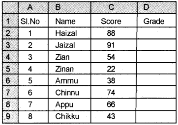
Step 3 – Enter the following formula in cell D2
= IF(C2 < 30, “FAIL”, IF(C2 < 40, “D+”, IF(C2 < 50, “C”, IF(C2<60, “C+”, IF(C2 < 70, “B”, IF (C2 < 80, “B+”, IF(C2 < 90, “A”, IF(C2 < 100, “A+”))))))))
Step 4 – Drag the formula to D9
Output:

Question 2.
The sales made by 6 salesmen during three months are given below. You are required to prepare a statement showing the total sales of each salesman and total sales of the firm.
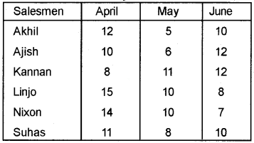
Procedure:
Step 1 – Open LibreOffice calc worksheet
Applications → Office → LibreOffice Calc
Step 2 – Enter the following data in the given cells
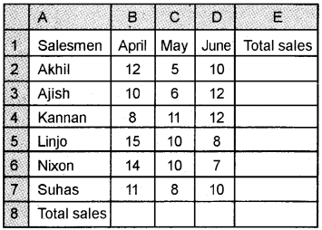
Step 3 – Enter the given formula in cell E2 = B2 + C2 + D2
Step 4 – Drag the formula to E7 to get the total sales of each salesman
Step 5 – Enter the given formula in cell E8 to get the total sales of the firm = SUM (E2: E7)
Output:

Question 3.
The monthly production of a company are given below
| Month | Production (Units) |
| January | 25000 |
| February | 20000 |
| March | 22000 |
| April | 18000 |
| May | 19000 |
| June | 24000 |
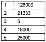
- Find the total production for the six months
- Find the average production of the six months
- Find the number of months during the period
- Find the lowest production of the six months
- Find the highest production of the six months
Procedure:
Step 1 – Open LibreOffice Calc worksheet
Applications → Office → LibreOffice Calc
Step 2 – Enter the following data in the given cells
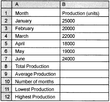
Step 3 – Enter the following formula in the given cells
| B8 | = SUM (B2:B7) |
| B9 | = AVERAGE(B2: B7) |
| B10 | = COUNT (B2:B7) |
| B11 | = MIN (B2:B7) |
| B 12 | = MAX (B2:B7) |
Output:
Question 4.
For the recruitment of managers in different departments of a company, Applicant’s age should be greater than 35 and less than 45 as on 31/03/2018. Write the Spreadsheet statement to test when a candidate is eligible for recruitment or not, when his/ her date of birth is entered in a cell as input
Procedure:
Step 1 – Open LibreOffice Calc Spread sheet.
Applications → Office → LibreOffice Calc
Step 2 – Enter the given data in the following cells
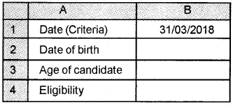
Step 3 – Enter the date of birth in cell B2
Step 4 – Enter the following formula in cell B3 = Round ((B1-B2)/365,0). Then the age will display in the cell B3.
Step 5 – Enter the following formula in cell B4 to test the eligibility of the candidate = IF(B3<35, “Not eligible”, IF(B3>45, “Not eligible”, “Eligible”)
OR
= IF (AND (B>34, B3<46), “Eligible”, “Not eligible”)
Note: The data value entered in cell B2 and B3 are to be formatted as “Date”
Question 5.
The given table shows name of employees, Designation and monthly salary paid for different employees in Jose Traders.
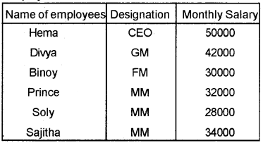
Find out the following:
- The total monthly salary by naming range (TOTAL SALARY)
- The total monthly salary paid to marketing managers (MM) in the firm
- The name of employees with a monthly salary of Rs.30000 by using LOOK UP function.
Procedure:
Step 1 – Open LibreOffice Calc worksheet
Applications → Office → LibreOffice Calc
Step 2 – Enter the data in the appropriate cells
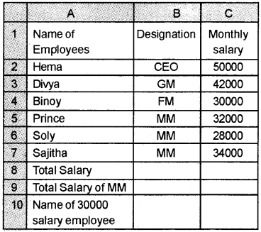
Step 3 – Naming a range
Select the range which shows monthly salary ie C2: C7 click on “Data” from the menu bar. Select “Define Range” Type the name “TOTAL_SALARY” in the name box and press OK or Enter key
Select the Range (C2: C7) → Data → Define Ranges Type TOTAL_SALARY. Press OK/Enter Key
Step 4 – Enter the following formulas in respective cells .
| B8 | = SUM (TOTAL_SALARY) |
| B9 | = SUMIF(B2:B7, “MM”, C2:C7) |
| B10 | = LOOKUP(30000, C2:C7, A2:A7) |
Output:

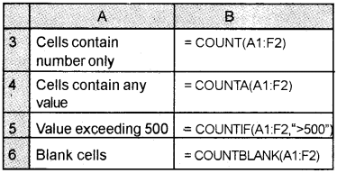
Question 6.
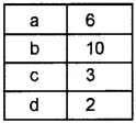
The following Data is given in the form of a Table.

- How many cells contain numbers only?
- How many cells contain any value?
- Count the number of cells containing the value exceeding 500.
- How many blank cells are there in the table?
Procedure:
Step 1 – Open LibreOffice Calc
Applications → Office → LibreOffice Calc
Step 2- Enter the given details in appropriate cells.

Step 3 – Enter the given details and formula in the Following cells.
Step 3 – Enter the given details and formula in the
Output:
Question 7.
The following details are given
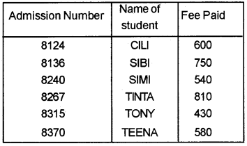
Find out
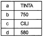
- Find the name of student whose admission number is 8267
- Look up value 8136 and locate the fee paid status by using VLOOKUP
- Look up the name of student against admission number 8124
- Ad. No. of student who paid fee Rs. 580
Procedure:
Step 1 – Open LibreOffice Calc worksheet
Application → Office → LibreOffice Calc.
Step 2 – Enter the details in the given cells
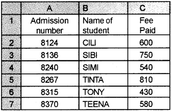
Step 3 – Enter the given details and formula in the following cells
| A | |
| 8 | Name of student Ad.No.8267 |
| 9 | Fee paid status of Ad No.8136 |
| 10 | Name of student Ad. No.8124 |
| 11 | Ad.No. of student, paid Rs.580 |
| B | |
| 8 | = LOOKUP(8267,A2:A7,B2:B7) |
| 9 | = VLOOKUP(8136,A2:C7,3,0) |
| 10 | = LOOKUP(8124,A2:A7,B2:B7) |
| 11 | = VLOOKUP (8370,A2:C7,3,0) |
Output:
Question 8.
The marks in Accountancy of some students are given below.
| Name | Mark |
| Priya | 89 |
| Indira | -ab- |
| Sindhu | 56 |
| Reny | 64 |
| Beena | 49 |
| Bindhu | 50 |
| Resmi | -ab- |
Calculate:
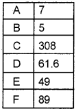
- Number of students in the class
- Number of students appeared in the Accountancy examination
- Total marks in Accountancy examination
- Average Marks in Accountancy examination
- Lowest mark in Accountancy
- Highest mark in Accountancy
Procedure:
Step 1 – Open LibreOffice Calc Work sheet
Application → Office → LibreOffice Calc.
Step 2 – Enter the given data in appropriate cells.
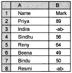
Step 3 – Enter the following details and formula in the given cells
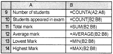
Output:
Question 9.
Mark summary of some students are given below.
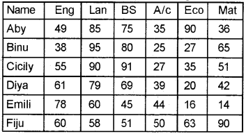
Calculate
- Number of cells containing 90 marks
- Count the number of paper scored less than 40
- Find the result of each student. (Pass or Fail) minimum mark required to pass is 30
Procedure:
Step 1 – Open LibreOffice Calc worksheet
Application → Office → LibreOffice calc
Step 2 – Enter the given data in appropriate cells
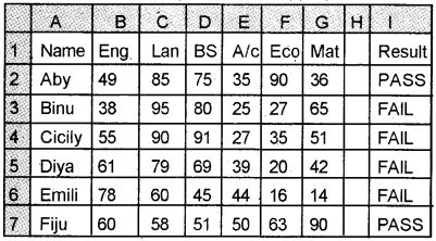
Step3 – Enter the following details and formula in appropriate cells
| A8 | Number of cells containing 90 mark |
| B8 | = COUNTIF(B2: G7, “90”) |
| A9 | Count the number of paper scored less than 40 Mark |
| B9 | = COUNTIF(B2: G7, “40”) |
Step4 – Find the result of the student
1ststep – Count the number of marks less than 30 scored by each student For this,
Enter the formula in H2 =COUNT IF (B2: G2, “<30”)
Drag the equation to H7
2nd step – Based on the result in H2: H7 range, we can find out the result in I2 cell by giving the following formula
=IF(H2 = 0, “PASS”, “FAIL”)
Drag (Copy) the formula to I7
Output:

Question 10.
List of debtors and creditors, and the amount due from them are given below
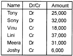
Calculate the total amount of receivables and payables using SUMIF functions.
Procedure:
Step -1 Open Libre Office Calc worksheet
Applications → Office → LibreOffice calc
Step 2 – Enter the details in the given cells.
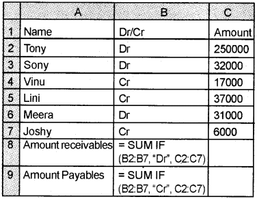
Output:

Question 11.
Calculate Income Tax of following employees based on the following criteria.
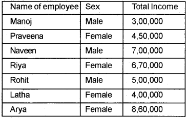
Conditions
- Tax rate is 40% of Total taxable Income.
- For male, standard deduction is 150,000 3 For female, if taxable income is less than or equal to Rs.4,00,000, then the standard deduction is 2,00,000, otherwise 1,50,000
Procedure:
Step 1 – Open LibreOffice Calc worksheet
Application → Office → LibreOffice calc
Step 2 – Enter the given details in the given range
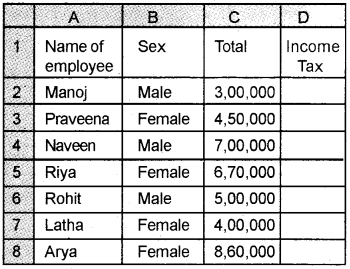
Step 3 – Calculation of Tax
Enter the formula in D2 cell and drag with the fill handle up to D8
= IF(B2 = “Male”, (C2 – 150000)*40%, IF (AND(C2 = “Female”, C2 <= 400000), (C2 – 200000)*40%, (C2 – 150000)*40%))
Output:
| Name of Employee | Tax |
| Manoj | 60,000 |
| Praveena | 1,20,000 |
| Naveen | 2,20,000 |
| Riya | 2,08,000 |
| Rohit | 1,40,000 |
| Latha | 80,000 |
| Arya | 2,84,000 |
Question 12.
For SI selection in Kerala polices there is a physical test, which consists of three items. A candidate has to qualify ANY ONE of the three tests to qualify for the final. The standard for the physical test is given below.
- Shot put: 5 meters or above.
- Ball throws 50 meters.
- 500-meter race within 5 minutes.
The following data is furnished:
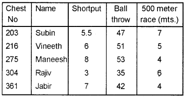
Check whether the candidates quality or not.
Procedure:
Step 1 – Open LibreOffice Calc worksheet
Application → Office → LibreOffice calc
Step 2 – Enter the details in the form of a Table
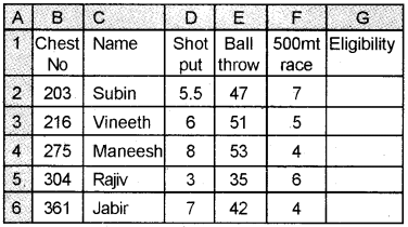
Step 3 – Enter the following formula in F2 and drag with fill up to F6 = IF(OR(C2>=5, D2>=50, E2<=5), ‘‘Qualified”, “Not Qualified”)
Output:
| Chest No. | Result |
| 203 | Qualified |
| 216 | Qualified |
| 275 | Qualified |
| 304 | Not Qualified |
| 361 | Qualified |
Question 13.
Calculate DAY, MONTH and YEAR of 36525 Procedure:
Step 1 – Open LibreOffice Calc worksheet.
Step 2 – Enter the details in appropriate cells.

Output:

Question 14. Calculate the Date value of 28/10/1978/
Procedure:
Step 1 – Open LibreOffice calc work sheet
Application → Office → LibreOffice Calc
Step-2 – Enter the given details in Cell A1 = DATEVALUE (“28/10/1978”)
Output:
![]()
Question 15.
Find the age of Resi Jos based on her date of birth and today’s date Date of birth 06-05-1981.
Procedure:
Step 1 – Open Libre office Calc work sheet Application officer LibreOffice calc
Step 2 – Enter the following details in appropriate cells.
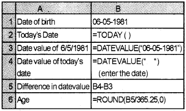
Output:
![]()
Question 16.
Below is given the table showing the name, department, and salary paid for different employees
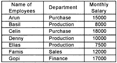
- Find number of employees in the firm.
- Find number of employees in Production Department.
- Find the total monthly salary paid in Purchase Department.
- Find the total monthly salary paid in Finance Department.
Procedure:
Step 1 – Open a new blank work sheet in LibreOffice Calc.
Step 2 – Enter the following details as given below.
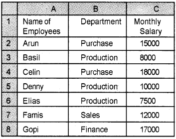
Step 3 – Enter the following text in different cells as given below.
| Cell | Text |
| A9 | No. of employees in the firm |
| A10 | No. of employees in the production department |
| A11 | Total monthly salary paid in purchase department |
| A12 | Total monthly salary paid in finance department |
Step 4 – Enter the following formula in different cells as given below.
| Cell | Formula |
| B9 | = COUNTA(A2: A8) |
| B10 | = COUNTIF(B2: B8, “Production”) |
| B11 | = SUMIF (B2: B8, “Purchase”, C2: C8) |
| B12 | = SUMIF (B2: B8, “Finance”, C2: C8) |
Output:
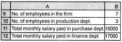
Question 17.
Below is given the table showing the Name, Department, and Salary paid for different employees.
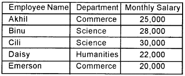
- Name the employee name column as “Emp Name”, Department column as “Dept” and monthly salary column as “Salary”.
- Find the total monthly salary.
procedure:
Step 1 – Open a blank worksheet in LibreOffice Calc.
Step 2 – Enter the following details in respective cells.
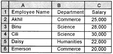
Step 3 – Select the range A2: A6, From the Data tool menu, select “Define Range” and – give name as “ Emp Name” and click (OK) button.
Step 4 – Select the range B2: B6, From the Data tool menu, select “Define Range” and give name as “Dept” and click (OK) button.
Step 5 – Select the range C2: C6, From the Data tool menu, select “Define Range” and give name as “Salary” and click (OK) button.
Step 6 – Enter the following formula to find out the total monthly salary.
| Cell | Text / Formula |
| A 7 | Total Monthly Salary |
| B 7 | = SUM (Salary) |
Output:
| Total Monthly Salary | 12500 |
Question 18.
Below is given the table showing the Name, Class, and Fees due to different students.
- Find out the total fees due from the students.
- Find the average amount of fees
- Find the highest amount of fees
- Find the lowest amount of fees
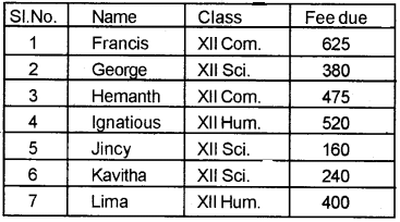
Procedure:
Step 1 – Open a new blank worksheet in LibreOffice Calc
Step 2 – Enter the following details in the worksheet as follows.
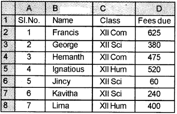
Step 3 – Enter the following text in respective cells.
| Cell | Text |
| A9 | Total Fees due |
| A10 | Average Fees |
| A11 | Highest amount of fees |
| A12 | Lowest amount of fees |
Step 4 – Enter the following formula in respective cells
| Cell | Formula |
| B9 | = SUM (D2: D8) |
| B10 | = Average (D2: D8) |
| B11 | = Max (D2;D8) |
| B12 | = Min (D2: D8) |
Output:
| Total Fees Due | 2700 |
| Average Fees | 386 |
| Highest Amount of Fees | 625 |
| Lowest Amount of Fees | 60 |
Question 19.
From the given values, calculate the following:
![]()
- Find the number of values
- Find the total sum of the values
- Find the average
- Find the largest value
- Find the smallest value
Procedure:
Step 1 – Open a new blank worksheet in LibreOffice Calc
Step 2 – Enter the values in the work sheet as follows.
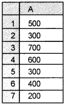
Step 3 – Enter the following text in the respective cells.
| Cell | Text |
| A8 | Number of values |
| A9 | Sum of the values |
| A10 | Average |
| AH | Largest value |
| A12 | Smallest value |
Step 4 – Enter the following formula in the respective cells.
| Cell | Formula |
| B8 | = COUNT (A1: A7) |
| B9 | = SUM(A1: A7) |
| B10 | = AVERAGE/A1: A7) |
| B11 | = MAX/A1: A7) |
| B12 | = MIN(A1: A7) |
Output:
| Number of values | 7 |
| Sum of the values | 3000 |
| Average | 429 |
| Largest value | 700 |
| Smallest value | 200 |
Question 20.
Prepare a statement showing advance tax collected form the employees @ 10% of the yearly salary from those who receive Rs. 500000 or more.
| Employees | Yearly salary |
| Fijo | 855000 |
| Joshy | 650000 |
| Roby | 720000 |
| Bose | 425000 |
| Prince | 570000 |
| Binoy | 380000 |
Procedure:
Step 1 – Open a new blank worksheet in LiberOffice Calc.
Step 2 – Enter the following details in the respective cells.
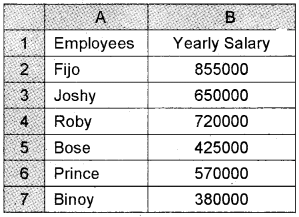
Step 3 – Select the range A2: A7, From Data Tools menu, select ‘Name a Range’ and give name as “Employees” and click (OK) button.
Step 4 – Enter the text /formula in the following cells.
| C | |
| 1 | Advance Tax |
| 2 | = IF (B2>=500000, B2*10%, 0) |
| 3 | |
| 4 | |
| 5 | |
| 6 | |
| 7 |
Step 5 – Copy formula to C3: C7 to the last employee.
Step 6 – Enter “Total Advance Tax” in cell B8 and enter the formula ‘‘SUM C2: C7” to get total amount.
Output:
| Fijo | 85500 |
| Joshy | 65000 |
| Roby | 72000 |
| Prince | 57000 |
Question 21.
Mrs. Leela, the class teacher is analysing the performance of her students in a class test.
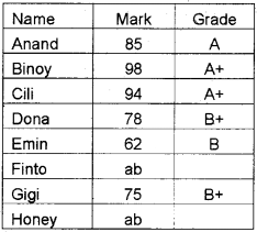
Find out
- Total number of students
- Number of students appeared in the class test
- Number of students with no grade
- Number of A+ holders
- Number of B grade holders.
Procedure:
Step 1 – Open a new blank worksheet in LiberOfficeCalc
Step 2 – Enter the following details in the respective cells.
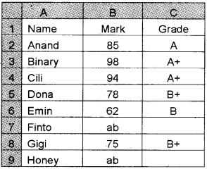
Step 3 – Enter the text /formula in the corresponding
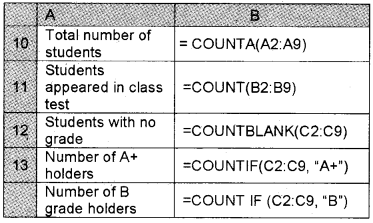
Output:
| Total number of students | 8 |
| Students appeared in-class test | 6 |
| Students with no grade | 2 |
| Number of A+ holders | 2 |
| Number of B grade holders | 1 |
Question 22.
The monthly sales effected by 6 salesmen are given below.
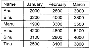
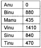
Calculate the commission earned by each salesman on the basis of the following rules.
| Total sales | Commission |
| Less than 8000 | Nil |
| 8000- 10000 | 5% |
| 10000- 12000 | 8% |
| More than 12000 | 10% |
Procedure:
Step 1 – Open a new blank worksheet in LibreOffice Calc.
Step 2 – Enter the following details in the respective cells.
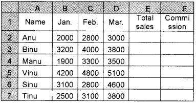
Step 3 – Enter the formula = SUM (B2: D2) in cell E2 to get the total sales. Copy the formula to the last employee.
Step 4 – Enter the formula = IF (E2 >= 12000, E2 * 10%, IF (E2 >= 10000, E2*8%, IF(E2 >= 8000, E2 * 5%,0)))
Copy the formula to the last employee.
Output:
Question 23.
ABC Ltd categorises their salesmen into four on the basis of sales targets achieved in each quarter. The criteria and sales are given below.
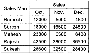
Performance criteria
Total sales – Grade
More than 100000 – Excellent
50000-100000 – Good
30000-50000 – Average
Less than 30000 – Bad
Procedure:
Step 1 – Open a new blank worksheet in LibreOffice Calc
Step 2 – Enter the following details in the respective cells.
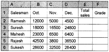
Step 3 – Enter the formula in E2 to get total sales = SUM (B2: D2)
Copy the formula to the last employee.
Step 4 – Enter the formula in F2 to get the commission = IF(E2 >= 100000, “EXCELLENT”, IF (E2 >= 50000, “GOOD”, IF (E2 >= 30000, “AVERAGE”, “BAD”)))
Copy the formula to the last employee.
Output:
| Ramesh | BAD |
| Suresh | GOOD |
| Mahesh | AVERAGE |
| Rajesh | GOOD |
| Sukesh | GOOD |
Question 24.
Below is given the name and address of some students. Combine and show details in an address format using CONCATENATE function.
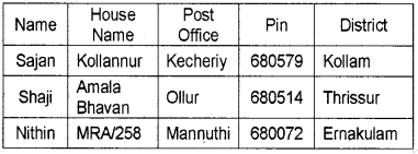
Procedure:
Step 1 – Open a new blank worksheet in LiberOffice Calc
Application → Office → LibreOffice Calc
Step 2 – Enter the following details in appropriate cells
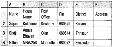
Step 3 – Enter the following formula in F2 cell = CONCATENATE (A2, “ ”, B2, “ ”, C2, “ ”, D2, “ ”, E2)
Step – 4 Copy down the formula up to the row of the last employee.
Output:
| Address |
| Sanjan Kollannur Kechery 680579. |
| Shaji Amala Bhavan Ollur 680514 Thrissur. |
| Nithin MRA/258 Mannuthy 680007 Ernakulam. |
Question 25.
Mr Venugoapl is planning to invest Rs. 10000 in the beginning of each year in an annual investment scheme. The interest rate is 8% and the term of the scheme is 10 years. Using FV function, find out how much amount he will get at the expiry of the scheme.
Procedure:
Step 1 – Open a new blank worksheet in LiberOffice Calc
Step 2 – Enter the given detials and formula in diffemt cells
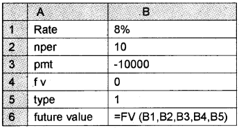
Output:
| Future value | 156454.87 |
Question 26.
Anakha Ltd. wants to select one machinery, out of the two alternatives available on the basis of net present value. The cost and inflows of these machineries are given below.
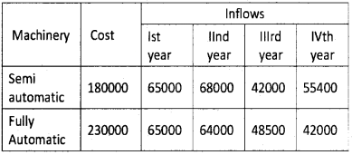
Assuming annual interest rate of 10%, find out net present values of these two machineries.
Procedure:
Step 1 – Open a blank work sheet in LiberOffice Calc
Step 2 – Enter the following details in respective cells.
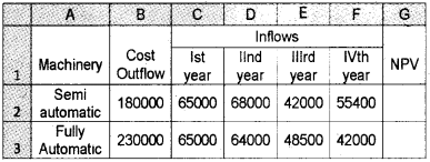
Step 3 – Enter the formula = NPV (10%, C2:F2) – B2 in G2 to get the net present value of semi automatic machinery.
Copy the formula to G3
Output:
| Machinery | NPV |
| Semi-Automatic | 4683.42 |
| Fully Automatic | 52891.2 |
Question 27.
Calculate Net Present Value (NPV) from the following data
| Cost of Machinery | 2000000 |
| Cash inflows -1 year | 60000 |
| Cash inflows – II year | 80000 |
| Cash inflows – III year | 82000 |
| Cost of capital | 12% |
Procedure:
Step 1 – Open a new blank worksheet in LibreOffice Calc
Step 2 – Enter the following details in the respective cells.
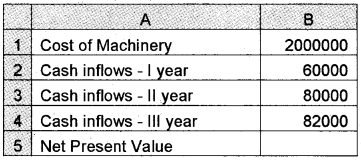
Step 3 – Enter the formula in B6 = NPV (12%, B2:B4)-B1 to get NPV
Output:
| Net Present value | 24287.08 |
Question 28.
Write the Libre Office Calc formula to multiply a given number entered in a cell with the following conditions
- If the cell value is less than 20, then multiply by 1
- If the cell value is greater than or equal to 20 but less than 40, then multiply by 2
- If the cell value is greater than or equal to 40 but less than 80, then multiply by 3
- If the cell value is greater than or equal to 80 but less than 100, then multiply by 4.
- If the cell value is greater than or equal to 100, then display “Enter a value less than 100” Use nested IF function.
Procedure:
Step 1 – Open a blank work sheet in LibreOffice Calc
Step 2 – Enter the following details in respective cells.
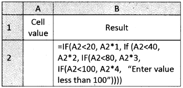
Step 3 – Enter any value in cell A2; then the result will be in cell B2.
Output:
| Cell value | Result |
| 18 | 18 |
| 37 | 74 |
| 115 | Enter value less than 100 |
| 85 | 340 |
Question 29.
Salary detail of 8 employees are given below.
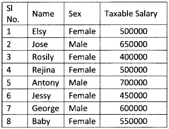
Develop a formula to compute tax under the following conditions.
1. Tax rate-20%
2. For males, Rs. 2,00,000 is allowed as standard deduction. For females, if taxable income is less than or equal to Rs. 5,00,000, then Rs. 3,00,000 is allowed as standard deduction, otherwise Rs. 2, 50,000. Use suitable logical function.
Procedure:
Step 1 – Open a new blank worksheet in LibreOffice Calc
Step 2 – Enter the following details in respective cells.
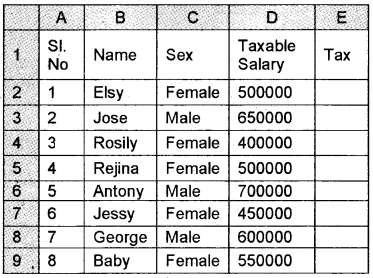
Step 3 – Enter the formula in cell E2 and copy it to the last employee.
=IF (C2 = “MALE”, (D2-20Q000)*20%, IF (AND(C2 = “FEMALE”, D2<=500000), (D2 – 300000) * 20%, (D2-250000)*20%))
Output:
| Name | Tax |
| Elsy | 40,000 |
| Jose | 90,000 |
| Rosily | 20,000 |
| Rejina | 40,000 |
| Antony | 1,00,000 |
| Jessy | 30,000 |
| George | 80,0000 |
| Baby | 60,000 |
Question 30.
The recruitment process of language teachers in a school consists of three items like interview, group discussion and paper presentation. A candidate has to qualify any one of the three tests to qualify for the written test. The prescribed standard for the items are given below.
- Interview – 16 score out of 20.
- Group Discussion – 25 score out of 30.
- Paper Presentation – 40 score out of 50
Other informations are also available.
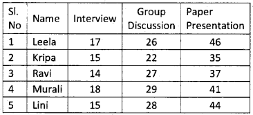
Write a formula using OR function to check whether a candidate qualify or not.
Procedure:
Step 1 – Open a blank work sheet in LiberOffice Calc.
Step 2 – Enter the available data in work sheet
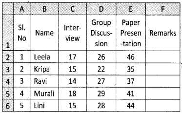
Step 3 – Enter the formula in F2 and copy it to the last candidate
= IF(OR (C2>=16, D2>=25, E2>=40) “Qualified for the written Test”, “Not Qualified”)
Output:
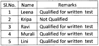
Question 31.
Business studies, Accountancy and Economics are commerce subjects. Write a formula to check whether text is a commerce subject. If yes, print **** is a commerce subject, otherwise print **** is not a commerce subject. Write procedure based on the available hints
Procedure:
Step 1 – Open a blank work sheet in LiberOffice Calc
Step 2 – Enter the text in the following cells.

Step 3 – Enter the name of subject in A2 and type the formula in B2 and drag it
= IF (OR (A2= “Business studies”, A2 = “Accountancy”, A2= “Economics”), A2 & “is a” & “Commerce Subject”, A2 & “is” & “not a commerce subject”)
Output:
| Subject | Remarks |
| Malayalam | Malayalam is not a commerce subject |
| Business studies | Business studies is a commerce subject |
| Chemistry | Chemistry is not a commerce subject |
| Mathematics | Mathematics is not a commerce subject |
| Accountancy | Accountancy is a commerce subject. |
Question 32.
ABC company issued a security with par value Rs. 50000 on 1/1/2013. The first interest date is 1-4-2013, the settlement date is 31-12-2015 an the annual coupon rate is 6%. The security’s payments are made quarterly, and a US (NASD) 30/360 day count basis is used. Use ACCRINT() function to calculated the accrued interest of a security that pays periodic interest.
Procedure:
Step 1 – Open a blank new worksheet in LibreOffice Calc.
Step 2 – Enter the data in the following cells.
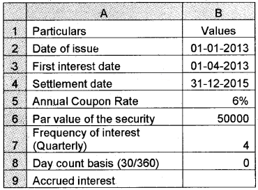
Step 3 – Enter the formula in B9 = ACCRINT (B2, B3, B4, B5, B6, B7, B8)
Output:
| Accrued Interest | 9000 |
Question 33.
Prince took a loan of Rs. 500000 from banks @ 12% interest p.a. repayable after 15 years. Compute interest payable at the end of (a) First year (b) Second year (c) Fifth year and the last year.
procedure:
Step 1 – Open a new blank worksheet in LibreOffice Calc
Step 2 – Enter the given details in respective cells
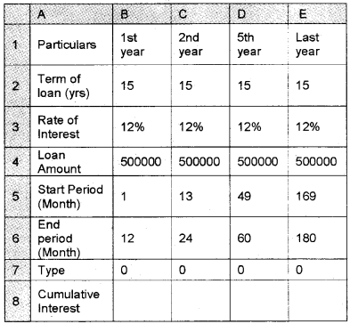
Step 3 – Enter the given formula in respective cells.
- B8 = CUMIPMT(B3/12, B2*12, B4, B5, B6, B7)
- C8 = CUMIPMT(C3/12, C2*12, C4, C5, C6, C7)
- D8 = CUMIPMT(D3/12, D2*12, D4, D5, D6, D7)
- E8 = CUMIPMT(E3/12, E2*12, E4, E5, E6, E7)
Output:
| Year | Interest |
| First year | 59316.92 |
| Second year | 57707.11 |
| Fifth year | 51545.84 |
| Last year | 4470.16 |
Question 34.
Calculate the present value of an annuity that pays Rs. 3000 per month for a period of 5 years. The interest is 11.5% per annum and each payment is made at the end of the month.
Assume the payments are made.
- At the beginning of each month
- At the end of each month
Procedure:
Step 1 – Open a new blank worksheet in LibreOffice Calc
Step 2 – Enter the following data/ Formula in respective cells.
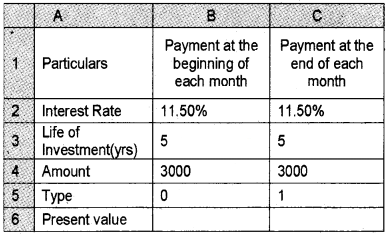
Step 3 – Enter the formula as follows
B6 = PV (B2/12, B3*12, B4, B5)
C6 = PV(C2/12, C3*12, C4, C5)
Output:
| Present value – at the beginning | 136409.4 |
| Present value – at the end | 136410.04 |
Question 35.
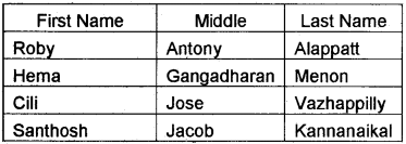
The table given below shows the First name, Middle name and Last name of some employees. Show their Full name in the next column using CONCATENATE Function.
Procedure:
Step 1 – Open a new blank worksheet in Liber Office Calc
Application → Office → Libre Office Calc
Step 2 – Enter the following details in appropriate cells
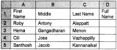
Step 3 – Enter the following formula in D2 cell = CONCATENATE (A2, “ ”, B2, “ ”, C2)
Step 4 – Copy down the formula up to the row of last employee.
Output:
| FULL NAME |
| Roby Antony Alappatt |
| Hema Gangadharan Menon |
| Cili Jose Vazhappilly |
| Santhosh Jacob Kannanaikal |
