What is Cumulative Frequency in statistics
- If the frequency of first class interval is added to the frequency of second class and this sum is added to third class and so on then frequencies so obtained are known as Cumulative Frequency (c.f.).
- There are two types of cumulative frequencies (a) less than, (b) greater than
- A table which displays the manner in which cumulative frequencies are distributed over various classes is called a cumulative frequency distribution or cumulative frequency table.
- There are two types of cumulative frequency.
(1) Less than type
(2) Greater than type
Read More:
- Classmark and Discrete Frequency Distribution
- RS Aggarwal Class 10 Solutions Mean, Median, Mode of Grouped Data
- RS Aggarwal Class 9 Solutions Statistics
Cumulative Frequency Table Example Problems with Solutions
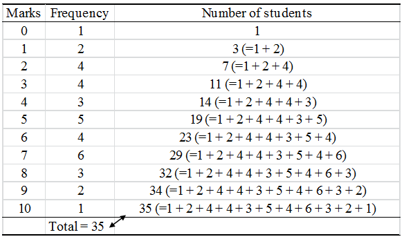
Example 1: The marks obtained by 35 students in a class are given below. Construct the cumulative frequency table :
| Marks obtained | Number of students |
| 0 | 1 |
| 1 | 2 |
| 2 | 4 |
| 3 | 4 |
| 4 | 3 |
| 5 | 5 |
| 6 | 4 |
| 7 | 6 |
| 8 | 3 |
| 9 | 2 |
| 10 | 1 |
Solution:
Example 2: The distribution of ages (in years) of 40 persons in a colony is given below.
| Age (in years) | Number of Persons |
| 20-25 | 7 |
| 25-30 | 10 |
| 30-35 | 8 |
| 35-40 | 6 |
| 40-45 | 4 |
| 45-50 | 5 |
(a) Determine the class mark of each class
(b) What is the upper class limit of 4th class
(c) Determine the class size
Solution: (a) Class marks are

= 22.5, 27.5, 32.5, 37.5, 42.5, 47.5
(b) The fourth class interval is 35–40. Its upper limit is 40
(c) The class size is 25 – 20 = 5
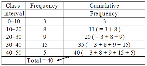
Example 3: Following is the distribution of marks of 40 students in a class. Construct a cumulative frequency distribution table.
| Marks | Number of Students |
| 0-10 | 3 |
| 10-20 | 8 |
| 20-30 | 9 |
| 30-40 | 15 |
| 40-50 | 5 |
Solution:
Example 4: The class marks of a distribution are 25, 35, 45, 55, 65 and 75. Determine the class size and class limit.
Solution: Class size = The difference between the class marks of two adjacent classes.
= 35 – 25
= 10
We need classes of size 10 with class marks as 25, 35, 45, 55, 65, 75
The class limits for the first class are
25 – 102 and 25 + 102
i.e. 20 and 30
First class is, therefore, 20–30
Similarly, the other classes are 30 – 40, 40 – 50, 50 – 60, 60 – 70, 70 – 80.
Example 5: Given below is the cumulative frequency distribution table showing the marks secured by 40 students.
| Marks | Number of Students |
| Below 20 | 5 |
| Below 40 | 10 |
| Below 60 | 25 |
| Below 80 | 32 |
| Below 100 | 40 |
Show in the class and their frequency form.
Solution:
| Marks | Cumulative frequency | Frequency |
| 0-20 | 5 | 5 |
| 20-40 | 10 | 5 ( = 10 -5) |
| 40-60 | 25 | 15 ( = 25 – 10) |
| 60-80 | 32 | 7 ( = 32 – 25) |
| 80-100 | 40 | 8 (= 40 – 32) |
Example 6: Write down less than type cumulative frequency and greater than type cumulative frequency.
| Height (in cm) | Frequency |
| 140 – 145 | 10 |
| 145 – 150 | 12 |
| 150 – 155 | 18 |
| 155 – 160 | 35 |
| 160 – 165 | 45 |
| 165 – 170 | 38 |
| 170 – 175 | 22 |
| 175 – 180 | 20 |
Solution: We have
| Height (in cm) | 140–145 | 145–150 | 150–155 | 155–160 | 160–165 | 165–170 | 170–175 | 175–180 |
| Frequency | 10 | 12 | 18 | 35 | 45 | 38 | 22 | 20 |
| Height Less than type | 145 | 150 | 155 | 160 | 165 | 170 | 175 | 180 |
| Cumulative frequency | 10 | 22 | 40 | 75 | 120 | 158 | 180 | 200 |
| Height Greater than type | 140 | 145 | 150 | 155 | 160 | 165 | 170 | 175 |
| Cumulative frequency | 200 | 190 | 178 | 160 | 125 | 80 | 42 | 20 |
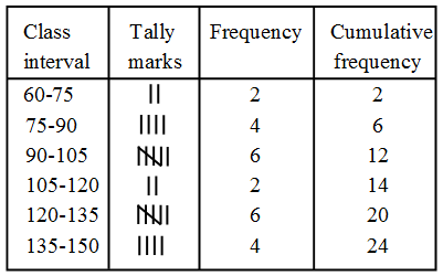
Example 7: The distances (in km) covered by 24 cars in 2 hours are given below :
125, 140, 128, 108, 96, 149, 136, 112, 84, 123, 130, 120, 103, 89, 65, 103, 145, 97, 102, 87, 67, 78, 98, 126
Represent them as a cumulative frequency table using 60 as the lower limit of the first group and all the classes having the class size of 15.
Solution: We have, Class size = 15
Maximum distance covered = 149 km.
Minimum distance covered = 65 km.
Range = (149 – 65) km = 84 km.
So, number of classes = 6 (since 8415 = 5.6
Thus, the class intervals are 60-75, 75-90,90-105, 105-120, 120-135, 135-50.
The cumulative frequency distribution is as given below :
Example 8: The following table gives the marks scored by 378 students in an entrance examination :
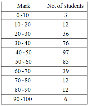
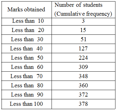
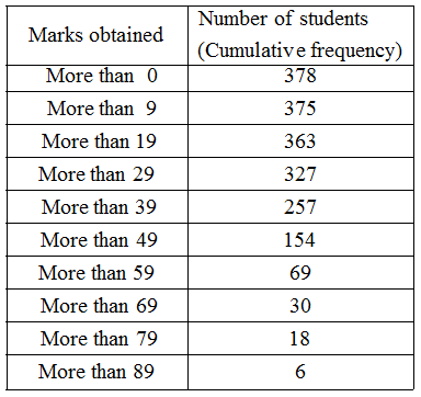
From this table form (i) the less than series, and (ii) the more than series.
Solution: (i) Less than cumulative frequency table
(ii) More than cumulative frequency table
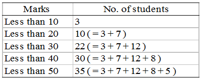
Example 9: Convert the given simple frequency series into a:
(i) Less than cumulative frequency series.
(ii) More than cumulative frequency series.
| Marks | No. of students |
| 0-10 | 3 |
| 10-20 | 7 |
| 20-30 | 12 |
| 30-40 | 8 |
| 40-50 | 5 |
Solution: (i) Less than cumulative frequency series
(ii) More than cumulative frequency series
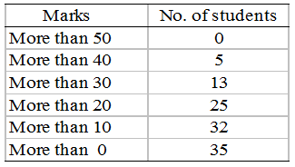
Example 10: Convert the following more than cumulative frequency series into simple frequency series.
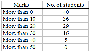
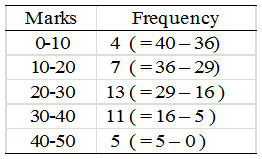
Solution: Simple frequency distribution table
Example 11: Drawn ogive for the following frequency distribution by less than method
| Marks | 0-10 | 10-20 | 20-30 | 30-40 | 40-50 | 50-60 |
| No. of Students | 7 | 10 | 23 | 51 | 6 | 3 |
Solution: We first prepare the cumulative frequency distribution table by less than method as given below :
| Marks | 0-10 | 10-20 | 20-30 | 30-40 | 40-50 | 50-60 |
| No. of Students | 7 | 10 | 23 | 51 | 6 | 2 |
| Marks less than | 10 | 20 | 30 | 40 | 50 | 60 |
| Cumulativefrequency | 7 | 17 | 40 | 91 | 97 | 100 |
Other than the given class intervals, we assume a class – 10-0 before the first class interval 0-10 with zero frequency.
Now, we mark the upper class limits (including the imagined class) along X-axis on a suitable scale and the cumulative frequencies along Y-axis on a suitable scale.
Thus, we plot the points
(0, 0), (10, 7), (20, 17), (30, 40), (40, 91), (50,97), and (60, 100)
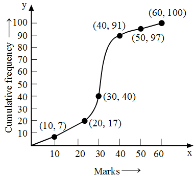
Now, we join the plotted points by a free hand curve to obtain the required ogive.
Example 12: Draw a cumulative frequency curve for the following frequency distribution by less than method
| Age (in years) | 0-9 | 10-19 | 20-29 | 30-39 | 40-49 | 50-59 | 60-69 |
| No. of persons: | 5 | 15 | 20 | 23 | 17 | 11 | 9 |
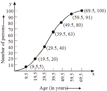
Solution: The given frequency distribution is not continuous. So, we first make it continuous and prepare the cumulative frequency distribution as under :
| Age (in years) | Frequency | Age less than | Cumulative frequency |
| 0.5 – 9.5 | 5 | 9.5 | 5 |
| 9.5 – 19.5 | 15 | 19.5 | 20 |
| 19.5 – 29.5 | 20 | 29.5 | 40 |
| 29.5 – 39.5 | 23 | 39.5 | 63 |
| 39.5 – 49.5 | 17 | 49.5 | 80 |
| 49.5 – 59.5 | 11 | 59.5 | 91 |
| 59.5 – 69.5 | 9 | 69.5 | 100 |
Now, we plot points (9.5, 5), (19.5, 20), (29.5,40), (39.5, 63), (49.5, 80), (59.5, 91) and (69.5, 100) and join them by a free hand smooth curve to obtain the required ogive as shown in Fig.
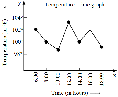
Example 13: The temperature of a patient, admitted in a hospital with typhoid fever, taken at different times of the day are given below. Draw the temperature-time graph to reprents the data:
| Time (in hours) | 6:00 | 8:00 | 10:00 | 12:00 | 14:00 | 16:00 | 18:00 |
| Temperature (in °F) | 102 | 100 | 99 | 103 | 100 | 102 | 99 |
Solution: In order to draw the temperature-time graph, we represent time (in hours) on the x-axis and the temperature in ºF on the y-axis. We first plot the ordered pairs (6, 102), (8, 100), (10, 99), (12, 103), (14, 100), (16, 102) and (18, 99) as points and then join them by line segments as shown in Fig.
Example 14: The graph shown in Fig. exhibits the rate of interest on fixed deposite upto one year announced by the reserve bank of india in different years. Read the graph and find.
(i) In which period was the rate of interest maximum?
(ii) In which period was the rate of interest minimum ?
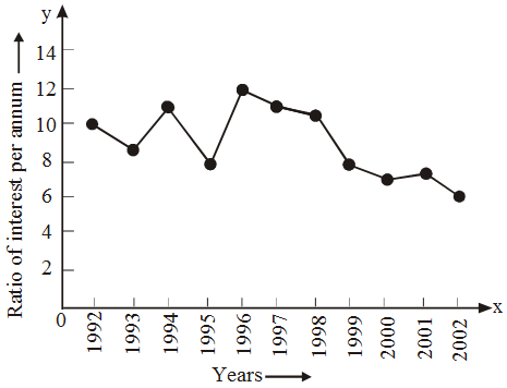
Solution: In the graph, we find that years are represented on x-axis and the rate of interest per annum is along y-axis. From the graph, we find that
(i) The rate of interest was maximum (12%) in 1996.
(ii) The minimum rate of interest was 6.5% in the year 2002.
Example 15: The following data represents the wages of 25 workers of a certain factory :
| Wages (in rupees) | No. of workers |
| 30-40 | 5 |
| 40-50 | 8 |
| 50-60 | 12 |
| 60-70 | 7 |
| 70-80 | 4 |
| 80-90 | 2 |
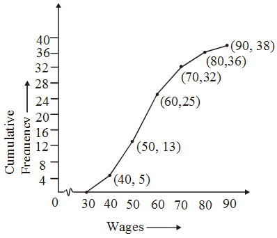
Solution: The cumulative frequency table is constructed as follows :
| Wages (in rupees) | No. of workers | Cumulative frequency |
| 30-40 | 5 | 5 |
| 40-50 | 8 | 13 |
| 50-60 | 12 | 25 |
| 60-70 | 7 | 32 |
| 70-80 | 4 | 36 |
| 80-90 | 2 | 38 |
The cumulative frequency curve is shown below:
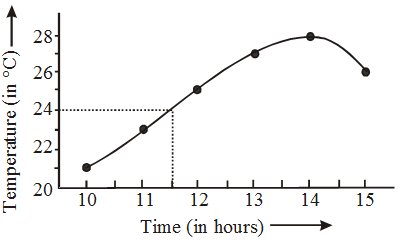
Example 16: Draw the Time-Temperature graph from the following table
| Time (in hour) | Temperature (in °C) |
| 10-00 | 21 |
| 11-00 | 23 |
| 12-00 | 25 |
| 13-00 | 27 |
| 14-00 | 28 |
| 15-00 | 26 |
From the graph estimate the temperature at 11-30 a.m.
Solution: Time in hours is denoted along the X-axis and temperature (in °C) is inidicated along the Y-axis. The points are joined by drawing a freehand curve. From the graph, the temperature at 11-30 a.m. is found to be 24.0°C.
